During this week week of July, the Amateur payload of DSLWP-B was active during the following slots:

• 14 Jul 19:00 to 21:00
• 15 Jul 12:00 to 14:00
• 17 Jul 04:40 to 06:50
• 18 Jul 20:50 to 22:50
• 20 Jul 14:20 to 16:20
• 21 Jul 05:30 to 07:30

Among these, the Moon was visible from Europe only on July 14, 18 and 21, so Dwingeloo only observed these days, which were mainly devoted to the download of SSDV images of the lunar surface. As usual, the payload took an image automatically at the start of each slot, so some of the slots were used for autonomous lunar imaging, even though no tracking was made from Dwingeloo.

This post is a detailed account of the activities done with DSLWP-B during the third week of July.

2019-07-14

On July 14, the payload was active between 19:00 and 21:00. DSLWP-B was behind Moon until 19:30, and when telemetry was first received, some problems were detected with the decoder at Dwingeloo. After some investigation, it was detected that the problems were caused by the tracking files in dslwp_dev. Usually, Wei Mingchuan BG2BHC generates the tracking files using STK, but he had some problems with the software and was unable to generate the files. Thus, I used GMAT to generate tracking files for the whole week.

I tried to use exactly the same format as in Wei’s tracking files, but I made a mistake in the zero padding of some fields. This caused problems with the Doppler correction code in the decoder. After disabling the Doppler correction, Dwingeloo was able to decode telemetry, but some time was lost trying to debug these issues.

First, image 0xF7, which was partially downloaded on July 12, was fixed by downloading the missing chunks. The download of this image started while Tammo Jan Dijkema was rushing to fix the Dwingeloo decoder. I ran a decoder in my computer through the Dwingeloo WebSDR, but unfortunately the WebSDR uses variable resampling that prevents successful decoding of a good fraction of the packets. While we attempted to transmit the missing chunks several times, Tammo Jan managed to fix the decoder at Dwingeloo, and image 0xF7 was completed. It is shown below. The image belongs to a series of four images of Mare Anguis taken on July 12.

After image 0xF7 was fixed, we downloaded image 0xF5, which is another of the images in the Mare Anguis series. This image took 40 minutes to transmit due to the large amount of detail present, which makes the JPEG file larger. Some of the chunks of the image were corrupted due to frequency jumps in the on-board TCXO.

After the download of this image finished, and with few minutes remaining until the payload shut down, the download of image 0xF6 (also in the Mare Anguis series) was started. The partial image received before shut down is shown below.

2019-07-18

The activation of July 18 was supposed to start at 21:50. However, the team from Dwingeloo were surprised when they started receiving telemetry just after pointing the dish, at 21:37. After examining the runtime field of the telemetry, it was discovered that the payload had powered on at 20:50 instead, so only a bit more than one hour of activation remained. Later it was discovered that the stated activation start of 21:50 was due to a mistake when converting from Beijing time into UTC.

The original plan for this activation was to download the image that was taken coinciding with the payload activation at 21:50. I had already computed that this image would show an area not far from the Apollo 15 landing site from an altitude of 143km, much lower than previous lunar surface images. However, after discovering that the payload had activated at 20:50, we realized that the image had been taken at 20:50.

I quickly run a GMAT simulation and checked that the lunar surface was not in the camera field of view at 20:50, so there wasn’t much point in trying to download that image. Instead, it was decided to take an image manually. Since the time was close to 21:50, this image would be similar to the prediction I had made.

After an unsuccessful try, Reinhard Kuehn managed to command the payload to take an image. This image was then downloaded without errors. It is shown in the figure below.

The figures below show the GMAT simulation for this image. See my previous post for more information about these simulations.

The GMAT simulation shows this area of the lunar surface, but I haven’t been able to recognize the features that appear in the image. Maybe someone can help? Keep in mind that the camera image is rotated, so that north is not the top of the image. Most likely, north is towards the right side of the image.

After the image was downloaded, it was planed to fix image 0xF5 shown above, by downloading the missing chunks. However, image 0xF4 was selected instead by mistake. This is the first image in the series of images of four images of Mare Anguis taken on July 12, which we also planned to download in the future. Since there were only 10 minutes until the payload shut down, we let the download continue instead of wasting time by cancelling the download. The partial image is shown below. It will be interesting to make a panorama with all the Mare Anguis images.

Another activity done on July 18 was attempting to command the B0 transmitter to send an SSDV image. The Amateur payload on DSLWP-B has two independent radios, B0 and B1, which work with different downlink and uplink frequencies. Usually, B1 is used to transmit the SSDV images, and B0 only transmits occasional GMSK and JT4G telemetry.

Having B0 and B1 transmit an SSDV image simultaneously in different frequencies (spaced 1MHz apart) would give very interesting possibilities for VLBI observations (see my conclusions to the 2018-11-21 VLBI experiment). However, this experiment hasn’t been performed yet due to worries of overheating the payload with both transmitters on for several minutes. Now that the mission of DSLWP-B has almost finished, this is no longer a concern.

Therefore, we tried to command the B0 radio to transmit an SSDV image while B1 was transmitting the images shown above. However, the radio didn’t seem to accept Reinhard’s commands. This will be tested again in the next activations.

2019-07-21

On July 21, the payload was active between 05:30 and 07:30 UTC. First, image 0xFF, which was taken at payload power on was downloaded. It was already known that the Moon was not visible in this image, so this image shows a faint field of stars. I haven’t managed to identify the image with astrometry.net. Probably there are not enough stars visible.

After downloading the field of stars, image 0xF4 was downloaded. Part of this image had been downloaded on July 18, but the image was downloaded again completely. The download succeeded without any lost chunks. This is one of the images in the Mare Anguis series.

Next, the download of image 0xFA was started. This image was taken at the payload activation on July 15 and it was supposed to show an area close to the Apollo 14 landing site. However, it was quickly seen that the image was a purple background, so the download was interrupted.

It is not completely known why this image doesn’t show the Moon surface, as it should according to the simulation. The leading theory is that the flywheels of DSLWP-B weren’t working properly when the image was taken, so the attitude of the satellite was different from the nominal. This makes sense, because the image is a purple background probably because it is over exposed due to the Earth being inside the field of view (or near it). However, with the nominal attitude the Earth shouldn’t be near the field of view of the camera, even if the image was taken at a different time.

The two figures below show the GMAT prediction corresponding to this image.

Finally, image 0xFD, which was taken at payload power on on July 20, was partially downloaded until the payload turned off at 08:30 UTC. According to the GMAT simulation, this image should show an area of the lunar surface around the Schlüter crater. For some unknown reason this image is purple, unlike most other lunar surface images, which are yellowish.

The figures below show the GMAT prediction for the image. In the field of view image, Schlüter crater is clearly visible towards the bottom right. The bottom part of the image shows the northern rim of Mare Orientale.

Below, I have marked the imaged area in Google Moon. The northeastern large crater is labeled as Riccioli P in this lunar chart, but I haven’t found any names for the other craters.

Lucky-7 is a Czech Amateur 1U cubesat that was launched on July 5 together with the meteorological Russian satellite Meteor M2-2 and several other small satellites in a Soyuz-2-1b Fregat-M rocket from Vostochny. The payload it carriers is rather interesting: a low power GPS receiver, a gamma ray spectrometer and dosimeter, and a photo camera.

It transmits telemetry in the 70cm Amateur satellite band using 4k8 FSK with an Si4463 transceiver chip. Additional details about the signal can be found here.

After some work trying to figure out the scrambler used by the Si4463, I have added a decoder for Lucky-7 to gr-satellites. This post shows some of the technical aspects of the decoder.

The framing used by Lucky-7 is really simple: the 16 bit syncword 0x2DD4 is followed by 35 bytes of data and 2 bytes of CRC-16. The data is scrambled using the default register settings for the Si4463.

In principle, that scrambler is a PN9 using the polynomial \(x^9 + x^5 + 1\) and seed 0x1FF. This should be similar to the scrambler of the TI CC1101 that I already have implemented as part of my Reaktor Hello World decoder. However, unlike Texas Instruments, which has detailed design note explaining the PN9 scrambler, I have not found good documentation from SiLabs for the Si4463 scrambler.

After trying out various things and reaching a dead end, I asked the Lucky-7 team if they could make me a recording of a Si4463 transmitting a scrambled packet whose payload is full of zeros. Such a packet shows the scrambling sequence directly. Jaroslav Laifr was kind enough to make a recording for me.

When analyzing Jaroslav’s recording, which had scrambled 64 byte frames full of zeros, I saw that the scrambling sequence is

87 b8 59 b7 a1 cc 24 57 5e 4b 9c 0e e9 ea 50 2a
be b4 1b b6 b0 5d f1 e6 9a e3 45 fd 2c 53 18 0c
ca c9 fb 49 37 e5 a8 51 3b 2f 61 aa 72 18 84 02
23 23 ab 63 89 51 b3 e7 8b 72 90 4c e8 fb c1 ff

I immediately recognized that sequence.

Recall that the TI PN9 scrambler is implemented in GNU Radio as shown in the figure below.

The bits per byte parameter is set to 8 because to scramble each byte, the 8 least significant bits from the scrambler shift register are taken, and then the shift register is shifted 8 times before scrambling the next byte. This produces the sequence

ff e1 1d 9a ed 85 33 24 ea 7a d2 39 70 97 57 0a 
54 7d 2d d8 6d 0d ba 8f 67 59 c7 a2 bf 34 ca 18 
30 53 93 df 92 ec a7 15 8a dc f4 86 55 4e 18 21 
40 c4 c4 d5 c6 91 8a cd e7 d1 4e 09 32 17 df 83  

You’ll recognize that sequence from the TI design note, where the first 512 bytes of the sequence are listed.

Another way, which is perhaps more common, to generate the scrambling sequence is to work in a bit by bit fashion. Thus, to scramble a bit of input, the least significant bit of the scrambler shift register is used, and then the shift register is shifted once before passing to the next bit. In GNU Radio, this is achieved by setting the bits per byte parameter of the Additive Scrambler block to 1 instead of 8 and feeding it unpacked bits (so that each byte contains only one bit of input).

When the PN9 polynomial is run in a bit by bit manner, it produces the following sequence:

ff 87 b8 59 b7 a1 cc 24 57 5e 4b 9c 0e e9 ea 50 
2a be b4 1b b6 b0 5d f1 e6 9a e3 45 fd 2c 53 18 
0c ca c9 fb 49 37 e5 a8 51 3b 2f 61 aa 72 18 84 
02 23 23 ab 63 89 51 b3 e7 8b 72 90 4c e8 fb c1 

You can also find this sequence in the TI design note if you read carefully: look at section 3.3 and take the least significant bit of each register state listed there.

You’ll notice that, except for the initial 0xff byte, this sequence is the same as the one that the Si4463 uses. So it seems that the Si4463 uses the same PN9 as the TI CC1101, but it runs it in a bit by bit manner instead of byte by byte, and skips the first output byte.

In GNU Radio, skipping the first output byte can be achieved by setting the seed value to the correct shift register state that the scrambler which starts by 0xff would have after having shifted out one byte. Taking into account the fact that the endianness of the shift register in GNU Radio is reversed (shifts are done to the left, instead of the right), this is 0x1e1. Note that 0xe1 is just 0x87, the second output byte, with the bits reflected (and the first 0x1 comes from the MSB of 0xb8).

Taking this into account, the Si4463 scrambler block in GNU Radio can be seen in the figure below. It takes unpacked bits as input and outputs packet bits.

It also turns out that the CRC-16 used by the Si4463 is the same that the CC1101 uses, so the CRC check block has been reused from the Reaktor Hello World decoder.

Some Lucky-7 frames decoded from a recording I made on July 7 are shown below.

0000: 80 20 00 00 00 00 00 00 00 00 00 00 00 00 00 00 
0010: 00 00 00 00 00 00 00 00 00 00 00 00 00 00 00 00 
0020: 00 00 00 

0000: 80 10 00 00 00 00 ff ff ff ff ff ff ff ff ff ff 
0010: ff ff 00 05 00 05 00 e4 0d 00 00 00 07 d1 07 d1 
0020: 07 d1 00

0000: 80 20 01 00 00 3c 00 00 00 00 00 00 00 00 00 00 
0010: 00 00 00 00 00 00 be 02 ce 00 0d 86 a0 00 00 00 
0020: e8 00 00 

0000: 80 10 01 00 00 3c 67 20 00 fb aa 09 01 23 c7 17 
0010: 1c 27 00 05 00 05 ba 16 12 21 af 40 07 d1 07 d1 
0020: 07 d1 00 

0000: 80 20 02 00 00 78 00 00 00 00 00 00 00 00 00 00 
0010: 00 00 00 00 00 00 be 3e d1 00 0d 00 67 03 00 00 
0020: e8 00 00 

0000: 80 10 02 00 00 78 68 20 01 07 aa 09 74 2c 93 14 
0010: 07 26 00 05 00 05 ba 16 10 21 af 40 07 d1 07 d1 
0020: 07 d1 00 

0000: 80 20 03 00 00 b4 00 00 00 00 00 00 00 00 00 00 
0010: 00 00 00 00 00 00 be 7a d1 00 0d 00 67 03 00 00 
0020: e8 00 00

0000: 80 10 03 00 00 b4 68 20 00 df aa 09 dd 15 1d 14 
0010: 03 26 00 05 00 05 b9 16 0f 21 af 40 07 d1 07 d1 
0020: 07 d1 00 

0000: 80 20 04 00 00 f0 00 00 00 00 00 00 00 00 00 00 
0010: 00 00 00 00 00 00 be b6 d1 00 0d 00 67 03 00 00 
0020: e8 00 00

Note that these frames do not follow the format given in the Lucky-7 protocol description. In particular, the callsign and satellite name are nowhere to be found. My guess is that the second byte is some sort of packet type indicator (0x10 or 0x20), and the third byte is a packet counter, which runs independently for each packet type. Let’s see if the satellite team can give more information about the format.

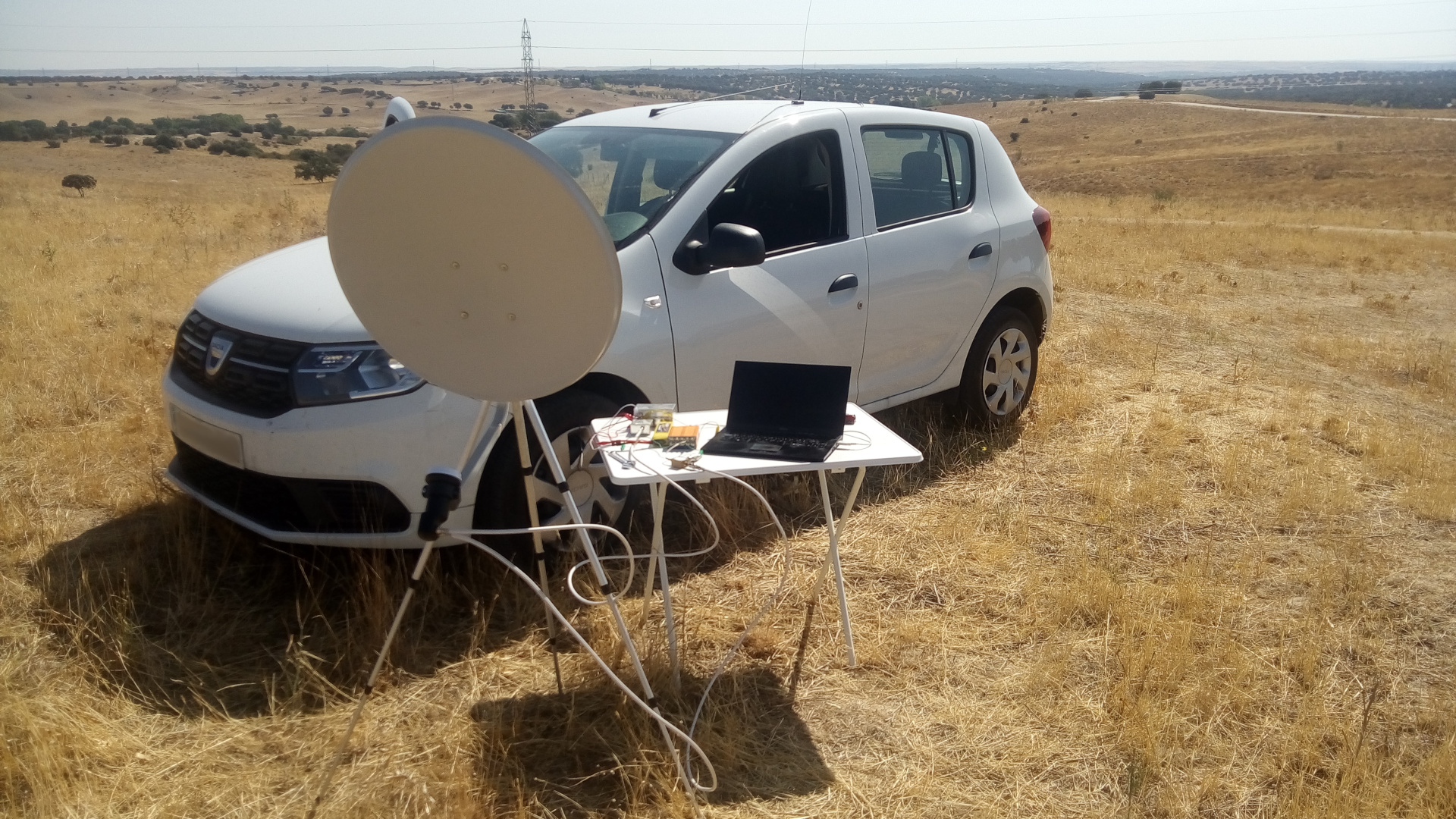
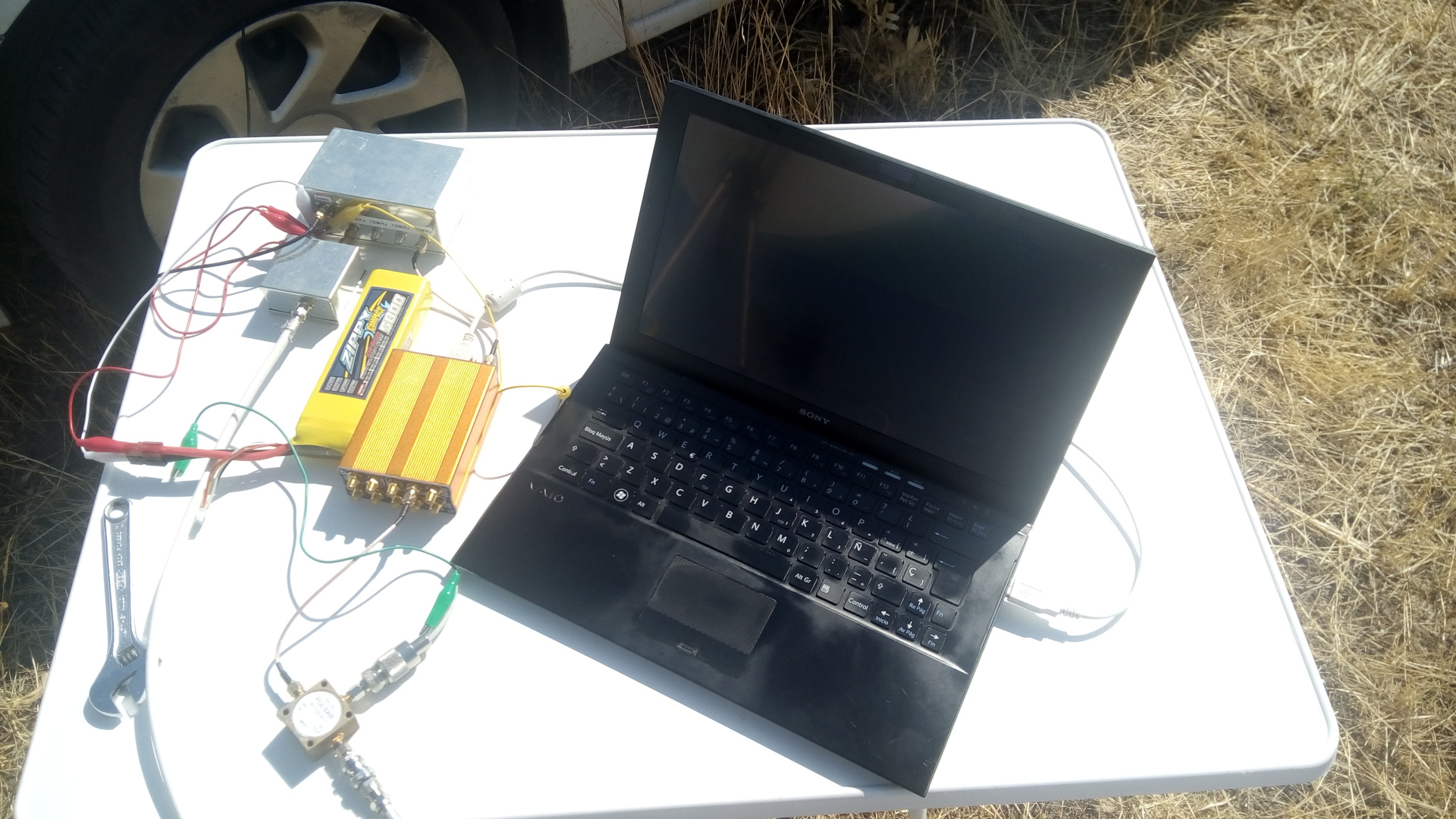
In May 25, the Moon passed through the beam of my QO-100 groundstation and I took the opportunity to measure the Moon noise and receive the Moonbounce 10GHz beacon DL0SHF. A few days ago, in July 22, the Moon passed again through the beam of the dish. This is interesting because, in contrast to the opportunity in May, where the Moon only got within 0.5º of the dish pointing, in July 22 the Moon passed almost through the nominal dish pointing. Also, incidentally this occasion has almost coincided with the 50th anniversary of the arrival to the Moon of Apollo 11, and all the activities organized worldwide to celebrate this event.

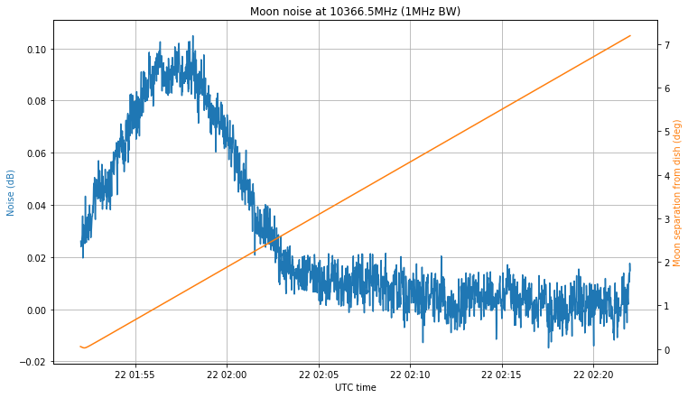
The figure below shows the noise measurement at 10366.5GHz with 1MHz and a 1.2m offset dish, compared with the angular separation between the Moon and the nominal pointing of the dish (defined as the direction from my station to Es’hail 2). The same recording settings as in the first observation were used here.

The first thing to note is that I made a mistake when programming the recording. I intended to make a 30 minute recording centred at the moment of closest approach, but instead I programmed the recording to start at the moment of closest approach. The LimeSDR used to make the recording was started to stream one hour before the recording, in order to achieve a stable temperature (this was one lesson I learned from my first observation).

The second comment is that the maximum noise doesn’t coincide with the moment when the Moon is closest to the nominal pointing. Luckily, this makes all the noise hump fit into the recording interval, but it means that my dish pointing is off. Indeed, the maximum happens when the Moon is 1.5º away from the nominal pointing, so my dish pointing error is at least 1.5º. I will try adjust the dish soon by peaking on the QO-100 beacon signal.

The noise hump is approximately 0.085dB, which is much better than the 0.05dB hump that I obtained in the first observation. It may not seem like much, but assuming the same noise in both observations, this is a difference of 2.32dB in the signal. This difference can be explained by the dish pointing error.

The recording I have made also covers the 10GHz Amateur EME band, but I have not been able to detect the signal of the DL0SHF beacon. Perhaps it was not transmitting when the recording was made. I have also arrived to the conclusion that the recording for my first observation had severe sample loss, as it was made on a mechanical hard drive. This explains the odd timing I detected in the DL0SHF signal.

The next observation is planned for October 11, but before this there is the Sun outage season between September 6 and 11, in which the Sun passes through the beam of the dish, so that Sun noise measurements can be performed.

SkyFox Labs is having some trouble identifying the TLE corresponding to their Lucky-7 cubesat. The satellite was launched on July 5 in launch 2019-038 and a good match among the TLEs assigned to that launch has not being found yet. Over on Twitter, Cees Bassa has analyzed some SatNOGS observations and he says that NORAD ID 44406 seems the best match. However, this TLE has already been identified by Spire as belonging to one of their LEMUR satellites.

Fortunately, Lucky-7 has an on-board GPS receiver, and the team has been collecting position data recently. This data can be used to match a TLE to the orbit of the satellite, and indeed is much more accurate than the Doppler curve, which is the usual method for TLE identification.

Jaroslav Laifr, from the Lucky-7 team, has sent me the data they have collected, so that I can study it to find a matching TLE. The study is pretty simple to do with Skyfield. I have obtained the most recent TLEs for launch 2019-038 from Space-Track and computed the RMS error between each of the TLEs and the GPS measurements. The results can be seen in this Jupyter notebook.

The best match is NORAD ID 44406, with an RMS error of 8.7km. The second best match is NORAD ID 44404 (which is what SatNOGS has been using to track Lucky-7), with an RMS error of 51.3km. Most other objects have an error larger than 100km.

Therefore, my conclusion is clear. It is very likely that Spire misidentified NORAD ID 44406 as belonging to LEMUR 2 DUSTINTHEWIND early after the launch, when the different objects hadn’t drifted apart much. NORAD ID 44406 is a good match for Lucky-7. It will be interesting to see what Spire says in view of this data.

Back in May, I spoke about the future collision of DSLWP-B with the lunar surface. It would happen on July 31, thus putting and end to the mission. Now that the impact date is near, I have run again the calculations with the latest ephemeris in order to have an accurate simulation of the event.

The ephemeris I’m using consist of a Moon centred ICRF Keplerian state vector which has been shared by Wei Mingchuan BG2BHC. In GMAT, this state vector is as follows:

DSLWP_B.Epoch = '25 Jul 2019 02:30:00.000';
DSLWP_B.CoordinateSystem = LunaICRF;
DSLWP_B.SMA = 8708.404;
DSLWP_B.ECC = 0.747921;
DSLWP_B.INC = 44.157;
DSLWP_B.RAAN = 52.405;
DSLWP_B.AOP = 86.261;
DSLWP_B.TA = 165.00062091131025;

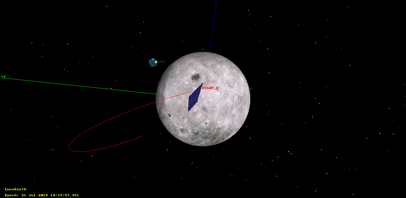
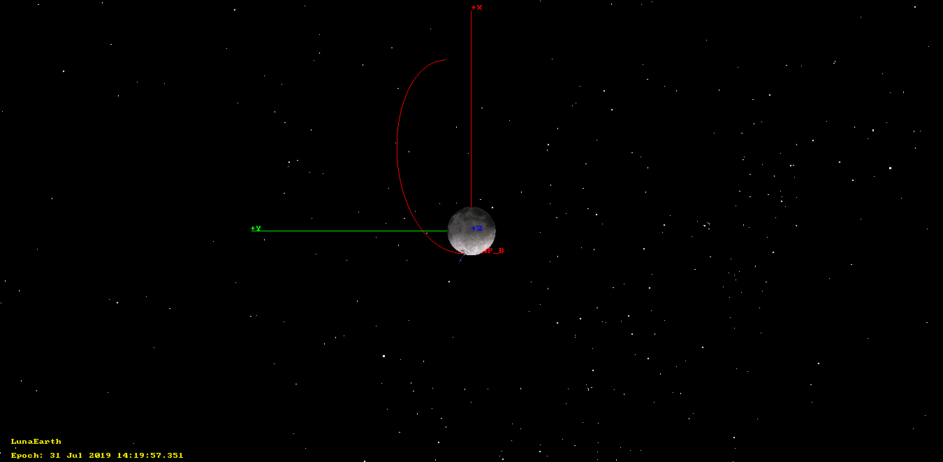
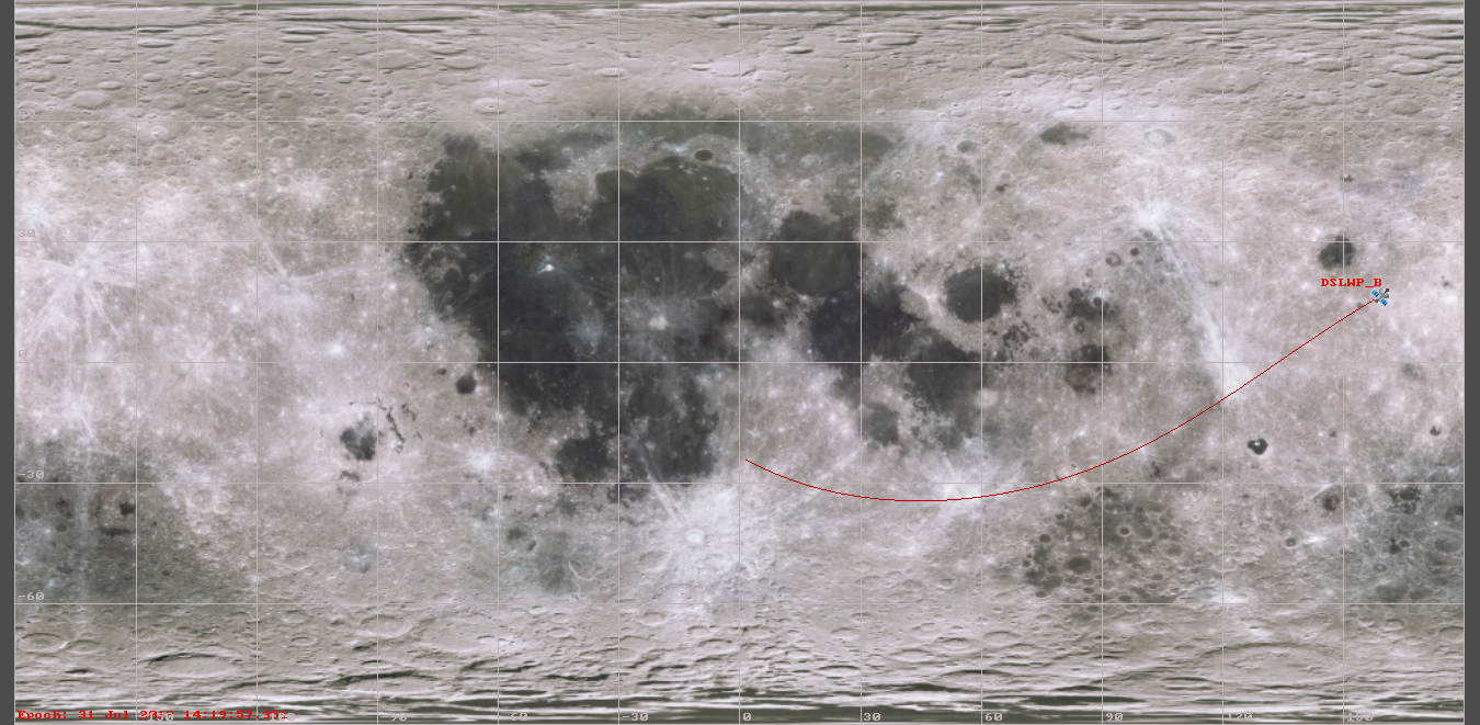
Using this GMAT script, I have obtained that the impact will happen on 2019-07-31 14:19:57 UTC, near Mare Moscoviense, in the lunar far side. This result is quite close to the calculations I did in May, which predicted an impact at 14:47 UTC.

The images below show the impact simulation in GMAT. Since the impact happens on the far side of the Moon, it will not be visible from Earth. There is an activation of the Amateur payload onboard DSLWP-B for 2019-07-31 13:24 to 15:24 UTC. The satellite will hide behind the Moon around 14:08 UTC. If the Moon was not solid, DSLWP-B would reappear around 14:35 UTC. The absence of radio signals after this moment will confirm that the impact has occurred.

During the fourth week of July, the Amateur payload on-board DSLWP-B was active in the following slots.

• 22 Jul 06:14 to 08:14
• 22 Jul 22:40 to 23 Jul 00:40
• 23 Jul 23:20 to 24 Jul 01:20
• 25 Jul 00:30 to 02:30
• 26 Jul 10:55 to 12:55
• 27 Jul 02:30 to 04:30
• 28 Jul 03:30 to 05:30

Additionally, Wei Mingchuan BG2BHC shared on Twitter the 10 minute slots for the activations of the X band transmitter. This transmitter uses a frequency of 8478MHz (in the Deep Space X band) and 2Mbps BPSK with CCSDS standards. The transmit power is 2W and the gain of the small X-band dish is 22dBi. The signal is detectable with small stations (as shown here), but to demodulate the data a large dish is needed. The Chinese DSN uses 35m and 50m antennas to receive this signal.

2019-07-22 morning

On July 22, the payload was active in two slots. During the first slot, from 06:14 to 18:14 UTC, first image 0x00, taken at payload power on, was downloaded. This payload shows a field of weak stars. Later, it was confirmed with GMAT that this was the expected field of view for the image.

I haven’t been able to identify the identify this image using astrometry.net. Probably there are too few stars for a reliable identification.

After downloading the field of stars, the missing chunks in image 0xF5 were fixed. This image belongs to a series of images of Mare Anguis taken one minute apart in July 12.

The satellite was programmed to take a series of four images with one minute spacing starting at 07:13, as the satellite passed through the perigee. However, since the payload was being commanded by VHF at that time, only the first image in the series was taken.

The payload accepts commands both by VHF and by RS-422 serial bus connected to the satellite bus, which is used to send commands previously programmed in the satellite using the S-band uplink. However, if the payload is currently transmitting an image using SSDV on the 70cm downlink, commands to take another image will be ignored, regardless of whether they are received over VHF or RS-422. This is what prevented the three last images in the series to be taken.

The image taken near the perigee was partially downloaded and then the download was stopped, since the original idea was to fix the missing chunks in image 0xFE instead.

The GMAT simulation shows that this image was taken as the camera was looking towards Oceanus Procellarum. A zoom factor of 4x instead of the usual 2x was tested with this image. This explains the relative lack of detail in the image.

An image was taken manually around 07:24. This image was downloaded later, but it only contains a purple field, so the download was stopped.

Finally, some of the missing chunks of image 0xFE, first downloaded last week, were fixed. With this, the image was almost complete.

2019-07-22 night

The second activation on July 22 was between 22:40 and 00:40. Dwingeloo was not active, since the time was quite late in Europe and the telescope operators needed some well deserved rest. The Asian stations in Harbin and Shahe (China), and Wakayama (Japan) were used as downlink. Uplink was provided, as usual, by Reinhard Kuehn DK5LA from Germany, who stayed awake despite the late time in Europe.

The first part of the activation was devoted to changing the camera zoom back to 2x, since it was decided that 4x gives worse results. After this, the missing chunks of images 0xFE and 0x01 were downloaded. First, some chunks of 0xFE were downloaded, then the missing chunks of 0x01, and finally the last remaining chunks of 0xFE.

Image 0xFE was identified last week as an area northwest of Schlüter crater. The resolution of this image is around 340m per pixel.

I have not attempted to identify image 0x01 shown below. It belongs to some area in the middle of Oceanus Procellarum, but due to the lack of detail, identifying the exact location is perhaps too difficult or impossible.

2019-07-23

On July 23, the payload was active from 23:10 to 01:20. Dwingeloo was active despite the late time in Europe. One of the activities planned for this slot was to switch the payload transmitter to an \(r=1/2\) Turbo code. Until October 2018, the DSLWP-B transmitters used 250baud with an \(r=1/2\) Turbo code. In October this was changed to 500baud with an \(r = 1/4\) Turbo code, which gives a similar decoding threshold, but performs better for VLBI observations.

Over the last few days, it was discussed to test the transmitter with 500baud and an \(r = 1/2\) Turbo code, which is twice as fast but needs 3dB more SNR for decoding. Since SNR is not a concern when using Dwingeloo to receive, but some of the latest images have taken up to 40 minutes to download, switching to \(r = 1/2\) seemed natural.

Since this is the first time that 500baud with \(r = 1/2\) was used, Wei had to make GNU Radio decoders for Dwingeloo. This decoders gave some small problems when they were first used.

At the start of the activation payload, with the transmitter still at \(r = 1/4\), the paload was commanded to download image 0x04, which was taken at the payload power on. This was used to have a continuous signal to test the decoders at Dwingeloo. The image turned out to be the purple field shown below. The download was stopped manually at 23:43 in order to let the payload execute a pre-programmed imaging as it passed the periapsis.

A series of four images with one minute spacing were taken starting at 23:45, as DSLWP-B passed through the periapsis. These images had IDs between 0x05 and 0x08. The camera view prediction in GMAT is shown below.

The area shown in the field of view of the camera is the western border of Oceanus Procellarum. The Ulugh Beigh and Lavoisier craters are visible near the centre of the image. Note that, in comparison with the perigee images of July 22, the view has shifted to the west, owing to the rotation of the Moon.

After the four images were taken, the last of them was downloaded. It shows an almost featureless area with a large crater in the bottom right corner. The corresponding area of the lunar surface will be identified below.

After having downloaded this image, the payload was switched to \(r=1/2\) at 00:21. Then, image 0x05 was downloaded. The Ulugh Beigh crater can be seen near the centre of the image, while a large portion of the Ulugh Beigh A crater is visible in the upper right corner. The difference in albedo and texture between the mare and the continental surface is clearly visible.

Next, image 0x07 was downloaded. It shows the Lavoisier C and T craters in the lower right corner (see this image), and another crater whose name I have not been able to find near the centre. Note that the upper left of this image overlaps the lower right of image 0x08, and the same crater can be seen in both images. The resolution of this image is approximately 280m per pixel.

2019-07-25

On July 25 the Amateur payload was active between 00:30 and 02:30. Dwingeloo and Reinhard were not active, due to the late time in Europe. The Asian stations served as downlink and uplink. First, the few missing chunks in image 0x07 were fixed.

After completing image 0x07, image 0x06 was downloaded. This image was the only remaining image from the series of four images taken as DSLWP-B passed the periapsis on July 23. It shows the Lavoisier C and T craters in the top left, Ulugh Beigh A near the centre, and Ulugh Beigh B and C toward the top right (see this image).

Now that the four images of the Ulugh Beigh and Lavoisier area are complete, Tammo Jan Dijkema has made a panorama fusing the four images in Hugin. The lower right image was the first image to be taken, and north is approximately on the left side of the panorama. Click the image to view it in full size.

2019-07-26

On July 26, the payload activation was between 10:55 and 12:55 UTC. A series of four images with one minute spacing was pre-programmed to be taken around 11:26, when the satellite was supposed to pass the periapsis. However, the programming was wrong due to a mistake with timezone conversions. The correct passage of periapsis was around 12:26.

Therefore, the first goal in this activation was to prevent DSLWP-B from taking the images programmed around 11:26. As I have mentioned above, the satellite cannot take images while an SSDV transmission is on. Therefore, the idea was to start the download of image 0xFE (which had already been downloaded) before 11:26.

Image number 14 in the buffer (which corresponded to 0xFE) was selected at 11:30. The download image command was sent at 11:20. After this, the download started and the payload hid behind the Moon between 11:32 and 12:16 approximately. Cees Bassa reported that the satellite was transmitting a JT4G message as it exited the occultation. This can be interesting to study diffraction (see this post).

After the satellite reappeared out of occultation, the idea was to send manually the commands to take images near the periapsis. However, only one of these commands was successful, resulting in the camera taking image 0x0B at approximately 12:29. This image was downloaded later, but for some unknown reason it is badly over-exposed, so it is impossible to identify any lunar surface features.

2019-07-28

On July 28 the payload was active between 03:30 and 05:30 UTC. After the payload turned on, image 0x0D, which was taken at payload power on, was downloaded. This image shows a few faint stars, in accordance with the GMAT prediction, in which the Moon was not in the field of view of the camera.

DSLWP-B would hide behind the Moon between approximately 04:16 and 04:55. To get a continuous signal during the occultation (which can be used to study diffraction), the team commanded the download of image 0xFE at 04:07. This image had already been completed at the beginning of the week.

As the satellite came out of the occultation and passed the periapsis, a series of four images was taken automatically between 04:54 to 04:57. The IDs corresponding to these images are 0x0E through 0x11. After the images were taken, the last of them was downloaded. It is shown in the figure below.

Next, the previous image in the series was downloaded. This image, which has an ID of 0x10, is shown below.

According to the GMAT simulation, the area corresponding to these images should be near Joule crater, in the far side of the Moon. In the figure below, which shows the camera view simulation, Sanford crater is clearly visible near the top of the figure. It is a double crater with the smaller Sanford C crater attached to the northern rim of the main crater.

I haven’t managed to identify the craters that appear in figures 0x10 and 0x11. They should be somewhere around Joule crater, but the few craters present in the image don’t look so remarkable that it’s easy to locate them in Google Moon. It is also interesting to note that there is little overlap among the two images (in comparison with the series taken on July 23). The two bright dots near the bottom right corner of 0x10 are also present in the top left of image 0x11.

A few days ago, I received a LimeRFE from Andrew Back of Lime Microsystems. He was kind enough to send me a unit so that I can test it and make some usage demos during the ongoing crowdfunding campaign at Crowd Supply.

The LimeRFE is intended to work as an RF frontend for the LimeSDR family, although it can work coupled with any other SDR or conventional radio. As such, it has power amplifiers, filters and LNAs designed to cover the huge frequency range of these SDRs. It is designed to cover all the Amateur radio bands from HF up to 9cm, and a few cellular bands.

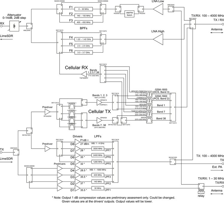
As anyone will know, designing broadband RF hardware is often quite difficult or expensive (Amateur radio amplifiers and LNAs are usually designed for a single band), so packing all this into a single unit is a considerable feat. The output power on most bands is around a couple watts, which is already enough for many experiments and applications. The block diagram of the LimeRFE can be seen below.

In this post I show a brief overview of the LimeRFE and demonstrate its HF transmission capabilities by showing a WSPR transmitter in the 10m band, using a LimeSDR as the transmitter.

The block diagram shown above refers to the LimeRFE 0v3 prototype that I got, so it doesn’t have specific hardware for the 6m, 4m, 1.25m and 33cm Amateur bands. Version 1v0, which is what the crowdfunding campaign backers will get, includes additional hardware for these bands. Support for these bands was added due to feedback from the community.

The schematics for 1v0 can be found here. Regarding the Amateur radio bands, for the receive side the work is split between two LNAs, an ADL5611 for the bands above 1GHz, and a GALI-74+ for the bands below 1GHz. There are specific bandpass filters for HF, 2m, 70cm, 23cm, 13cm and 9cm. For the transmit side there are individual PAs with lowpass filter for HF (RD16HHF1), 2m (AFT09MS007N), 1.25m (AFT09MS007N), 70cm (AFT09MS007N), 33cm (RFM04U6P), 23cm (RD01MUS2B), 13cm (QPA9426) and 9cm (MAAM-009560). The 6m and 4m bands use the HF PA and a 70MHz lowpass filter. There are also broadband PAs covering 1MHz-1GHz (RD01MUS2B) and 1GHz-4GHz (MAAM-009286), but these have somewhat lower power and no filtering. I haven’t found what MMICs are used as LNAs

The control of the LimeRFE is done either through USB from a host computer or through I2C from a LimeSDR. So far I only have used USB, as it is easier to set up. The control functions are integrated in the LimeSuite drivers (in the LimeRFE branch) and all the functionality can be controlled through the LimeSuiteGUI software, which is a quick and simple way to get the LimeRFE up and running. There are also some examples in C++ and Python that show how to use the drivers directly to control the LimeRFE.

The LimeRFE needs 12V DC power. This should be supplied through a 5.5mm OD, 2.5mm ID barrel jack connector. I thought that I had several of these lying around, but it turns out that all of them are for 2.1mm ID, and don’t fit the LimeRFE. The 2.5mm ID connector is also used in the LimeNET Micro, so they have kept the same connector for consistency. Fortunately, it is also possible to supply 12V through a pin header, which is what I’m doing.

It is recommended to have some SMA 50 Ohm terminations to prevent damage to the unit by having un-terminated ports (keep in mind that due to the presence of both PAs and LNAs, almost all the SMA connectors of the LimeSDR are a potential output). Up to 5 SMA terminations might be needed, but in many cases it is possible to get by with two or three terminations, since some of the LimeRFE ports will already be connected to a 50 Ohm load, such as an SDR or an antenna. In any case, terminating the ports is not completely mandatory. It is just useful to prevent damage due to configuration mistakes.

To test the LimeRFE as an HF transmitter, I have used a LimeSDR to generate the signal and the SDRangel software to drive the LimeSDR. Since the LimeRFE only has a 30MHz lowpass filter for HF, I have decided to work in the 10m band. For the lower bands, an external lowpass filter is needed to attenuate harmonics.

I have decided to use WSPR because it is a nice unattended mode that works well with low power.

The figure below shows the voltage at the LimeRFE output when connected to a 50 Ohm load. The RMS voltage is around 4.1V, which corresponds to 25dBm. This is significantly less than the 33dBm that the unit is supposed to deliver. I don’t know what the problem is. According to the engineers at Lime Microsystems, they get 33dBm with a LimeSDR mini, so this is surely a hardware problem that I will start debugging soon (either the output power of my LimeSDR in HF is too low or the LimeRFE was damaged on transport).

The antenna I am using is a long wire (approximately 15m long) in a urban location. This is my usual HF antenna at home and I have used it in most of my other HF experiments.

The nontrivial part about getting the WSPR transmitter running is controlling the PTT of the LimeRFE, or in other words, switching the LimeRFE between transmit and receive. I am using WSJT-X to generate the WSPR signal and send it by Pulseaudio to SDRangel. However, none of these programs knows how to control the LimeRFE.

Since this is was intended as a quick test, I have made a rather hackish solution: WSJT-X is configured to transmit with a 100% duty cycle, and the LimeRFE PTT is controlled through a standalone Python script that implements the desired duty cycle. For simplicity, a 50% duty cycle has been used.

The Python script gets the UTC time every second, decides whether the PTT should be enabled or not according to the duty cycle (2 minutes on, 2 minutes off, etc.), and sends a command to the LimeRFE accordingly. The Python script, which is based in the LimeRFE driver Python example can be seen here. It shows how easy it is to use the LimeRFE through Python. Note that, for simplicity, the initial settings of the LimeRFE (i.e., setting the band to HF) have been done with LimeSuiteGUI, but it would be quite easy to include this also in the Python script.

Of course, this solution is just a hack. The good solution would be to make a Python script that behaves as a Hamlib server and controls the LimeRFE accordingly. In this way, the LimeRFE could be interfaced easily with WSJT-X and other software supporting Hamlib. The example Hamlib Python server by Jim Ahlstrom N2ADR can be used as starting point.

The heatsink gets hot (approximately 55ºC) during extended operation with a 50% WSPR duty cycle, and output power seems to drop slightly as the temperature increases, so a small fan might be helpful. The engineers at Lime Microsystems tell me that there is a connector for a fan in the LimeRFE, and that sensing and controlling the fan is supported by the hardware, although this hasn’t been implemented in the drivers yet. The LimeRFE consumes an additional current of 1.7A at 12V when it goes from RX into TX (with the power and band settings of this WSPR experiment).

The WSPR transmitter experiment started at 2019-07-29 22:00 UTC and ended at 2019-07-31 16:20. During this time, the following spots have been reported by WSRPnet. The map of spots is shown in the figure below.

Besides doing some tests in HF, I have also tested the output power in the 2m and 70cm bands, also using a LimeSDR as transmitter. The results can be seen in this tweet. The transmit power is slightly above 3W, completely in line with the preliminary specifications, which give an output power of 33dBm (2m) and 32dBm (70cm) at 1dB compression. This is comparable to the 5W of a typical handheld or QRP radio, so it seems that a LimeSDR plus a LimeRFE is already able to be used for real world Amateur radio activities, and not just as lab equipment.

So far I am liking the LimeRFE and I think that the concept is a great idea. One of the reasons why I like my Yaesu FT817ND is that it is an all mode radio covering “all” the bands from HF to 70cm with 5W of power (not the 4m band, though). This is enough to perform many experiments and activities, and having all these bands inside a single unit is very convenient for the experimenter who wants to try many different things. The LimeRFE goes in the same direction: a few watts of power on “all” bands from HF to 9cm.

Besides its use below 1GHz, it is quite interesting for the microwave bands. Currently it is not so easy to become active on the microwave bands, since usually each band needs separate hardware including a PA, LNA and RF switch. The LimeRFE supports the three lower microwave bands with adequate power for many portable experiments, activations and contests. I think it can be a useful tool to encourage activity in these bands.

The only deterrent may be its price. At $600 during the crowdfunding campaign and $700 afterwards, it is something considerable, especially if you compare it with the price of a LimeSDR mini, which only costs $160. However I completely understand the reason for this price. RF hardware is usually expensive and supporting that many different bands inside one product makes it even more expensive.

I guess that if one was to purchase standalone amplifiers, LNAs and filters to achieve a similar functionality to the LimeRFE, the total cost would be much higher than $700. Therefore, I think that getting a LimeRFE can be a wise investment for many people interested in experimenting with SDRs and using them in real world scenarios, where at least a few watts of power, and perhaps some RX filtering, are often needed.

As probably you all know, the Chinese Amateur lunar orbiting satellite DSLWP-B was expected to collide with the Moon on July 31 at 14:20 UTC, so this is the last report about the DSLWP-B activities. The collision was planned since January this year, and was done as a means to end the mission without leaving debris in lunar orbit.

The activation slots for the Amateur payload on-board DSLWP-B for this week were the following:

• 29 Jul 00:15 to 02:15
• 29 Jul 04:30 to 06:30
• 29 Jul 20:00 to 22:00
• 30 Jul 05:30 to 07:30
• 30 Jul 16:20 to 18:20
• 31 Jul 06:30 to 08:30
• 31 Jul 13:24 to 15.24
• 1 Aug 05:30 to 07:30

I had calculated a periapsis height of -62km for the July 31 orbit, so the collision with the Moon was quite certain, even taking orbit errors into account. However, a slot was set on August 1 just in case the collision didn’t happen.

This post summarizes the activities done this week with DSLWP-B and the end of the mission.

2019-07-29

On July 29, the first activation was between 00:15 and 02:15 UTC. Only the Asian stations in Shahe and Harbin, China, and Wakayama, Japan, joined this observation, since it was rather late at night for European stations.

A series of four images with one minute of spacing was scheduled to be taken as the satellite passed the periapsis, at around 01:14. These images had IDs 0x13 to 0x16. The figures below show the GMAT simulation for this periapsis passage.

All the periapsides during these days happened northeast of Jackson crater, with the periapsis point shifting slightly to the west as time passed due to the rotation of the Moon. I haven’t attempted to identify any of the images, since the do not show any craters that might be easily recognizable.

After the periapsis passage, first, the last image of the series was downloaded. A few chunks were lost.

Next, image 0x13, the second of the series, was downloaded completely.

Then, image 0x15, the third in the series was downloaded. No chunks were lost, but the Amateur payload shut off at 02:15, before the whole image had been transmitted.

It is interesting to note that this image is yellowish, in contrast with the other images in the series, which have a purple hue. All the images were taken near the same time and area. It seems that a small difference in lighting conditions can trigger rather different auto-exposure settings, giving different hues to the image.

The next activation on July 29 was between 04:30 and 06:30. This time, the tracking was done by the European stations: the 25m radiotelescope at Dwingeloo,the Netherlands, which is the main downlink station, and Reinhard Kuehn DK5LA, in Germany, who is the main uplink station.

First, image 0x0F was downloaded. This image was taken during the periapsis passage on July 28. It has a brownish hue, in contrast with images 0x10 and 0x11, which are purple and were taken nearly at the same moment. These two other images were downloaded last week.

Next, image 0x0E, which was the first in the periapsis passage of July 28, was downloaded.

Finally, image 0x13 was downloaded. This was the first image in the series taken on the periapsis passage of July 29.

The last activation on July 29 was between 20:00 and 22:00 UTC, but the Moon was not visible in Europe and no Asian stations were able to track, so no activities were made during this slot. However, the satellite took at series of four images, with one minute spacing and IDs between 0x19 and 0x1C during the periapsis passage at around 21:35 UTC. The periapsis altitude was 114km. The figures below show the GMAT simulation for the camera view and ground track.

2019-07-30

The first activation on July 30 was between 05:30 and 07:30 UTC. Since this was early in the morning in Europe, it wasn’t possible to find the two operators that are needed to run the Dwingeloo radiotelescope. The tracking was done by the Asian stations and Reinhard DK5LA.

First, image 0x1B was downloaded. This is the third image corresponding to the second periapsis passage on July 29. A few chunks were lost.

Next, the previous image, with ID 0x1A, was downloaded. Again, a few chunks were lost.

After this, image 0x15, which was cut short in a previous activation as the payload turned off, was completed.

Then, image 0x1C, the last in the second periapsis passage on July 29, was downloaded, with some lost chunks near the beginning of the image.

Finally, image 0x19, the first in the second periapsis passage of July 29, was downloaded. The packet loss near the end of the image was quite severe, and after this image, the payload went off.

The second activation of the Amateur payload on July 30 was between 16:20 and 18:20 UTC. Dwingeloo was active but unfortunately the radio equipment there was suffering some problems that made the SNR of the DSLWP-B signals quite weak. The cause of the problem could not be found quickly, but at 16:52 the operators discovered that inserting a 20dB attenuator before the receiver seemed to improve things. This made us suspect that the problem was saturation due to out of band interference, but I am not sure if the real cause has been found. Fortunately, no problems appeared in subsequent observations.

The 20dB attenuator provided a workaround for the problem, and image 0x19 could be completed.

The Moon elevation in Europe was quite low, so Reinhard had problems pointing the antenna due to obstructions. Also, the satellite would hide behind the Moon between 17:38 and 18:07. Therefore, it was decided to stop commanding the satellite after image 0x19 was downloaded. However, Dwingeloo remained recording until the satellite hid below the horizon.

As the satellite hid behind the Moon, it passed the periapsis at 17:58 UTC. A series of four images with one minute spacing and IDs 0x1F to 0x22 were taken during the passage. The periapsis altitude was only 13km, so there was a special interest in downloading these close up views of the lunar surface. The figure below shows the ground track simulation in GMAT (nothing can be seen in the camera view simulation, since the resolution of the lunar surface imagery I’m using in GMAT is not high enough).

2019-07-31

The first activation on July 31 was between 06:30 and 08:30. Both the European and Asian stations were active. First, image 0x21, taken during the last periapsis passage was downloaded.

Then, image 0x20, the preceding image in the periapsis passage series was downloaded.

After this, image 0x22, the last of the July 30 periapsis passage was downloaded. A few chunks were lost and were downloaded later, at 07:44.

Then, image 0x1F, the first in the series taken during the July 30 periapsis passage was downloaded. Remarkably very few lost chunks were lost in these images, and indeed three were downloaded without packet loss. It is also impressive how many images have been downloaded during the last few days, helped by the change to 500baud and \(r = 1/2\), which give a bitrate of 250 bits per second.

Finally, image 0x1E, which was taken as the payload switched on during the second activation of July 30, was downloaded. This image shows a lense flare, cause by the camera being over-exposed by the Earth, which happened to be present at the lower right corner of the image.

The second activation on July 31 was between 13:24 and 15:24. This was a very emotive moment, since the collision with the Moon would happen during the activation, so it marked the end of the Amateur activities with DSLWP-B. Many people from the DSLWP-B team gathered on the HB9Q logger, where activations are usually coordinated.

The satellite would hide behind the Moon at around 14:08, with the collision happening at 14:20. Assuming that the ephemeris were somehow wrong and the collision didn’t happen, the satellite would reappear at 14:35. The tracking continued until it was determined that no signals were being received after 14:35, thus confirming that the collision had happened.

Cees Bassa twitted in real time the important moments of this activation. Edgar Kaiser DF2MZ was tracking the S-band beacon of DSLWP-B from Germany and also showed the loss of signal as the satellite hid behind the Moon to never appear again.

Before the satellite hid behind the Moon, it was possible to download a last image. This was image 0x24, which was taken at 13:24, as the Amateur payload powered on. It shows an over-exposed Earth.

As DSLWP-B hid behind the far side of the Moon, it was looking back to the Earth, the place where we all live, and we managed to grab this last view of our planet.

Downloading this image was not a trivial task, since a huge thunderstorm was ongoing near Reinhard’s station. This made it a difficult, and perhaps risky, task for Reinhard to command the satellite.

After 14 months, the DSLWP-B mission has now come to an end. This doesn’t mean that it is the end of my posts about DSLWP-B, since there are still lots of recorded data to process and studies to make.

I want to take this opportunity to thank all the people that have accompanied me in the amazing journey of DSLWP-B’s mission: The Chinese team, Wei Mingchuan BG2BHC, who has been leading the Amateur mission, Jizhuang Ma, who has been in charge of the station at Wakayama University, Sora KG5TEP, who made the Inory eye camera, and the rest of the people from Harbin Institute of Technology; Cees Bassa, Tammo Jan Dijkema, Jan van Muijlwijk PA3FXB, Paul Boven PE1NUT, Harry Keizer PE1CHQ, and the rest of the Dwingeloo team; Reinhard Kuehn DK5LA, who has always been there when uplink was needed; and many other Amateur radio operators who have engaged with the mission in one way or another (most of them are listed here).

In my last posts about DSLWP-B, I have been showing all the images of the lunar surface that were taken by the satellite during the last weeks of the mission, and tried to identify to which area of the Moon each image corresponded. For several of them, I was able to give a good identification using Google Moon, but for many of the latest images I was unable to find an identification, since they show few or none characteristic craters.

Thus, for these images I only gave a rough prediction of which area of the Moon was imaged by using GMAT and the published ephemeris from dslwp_dev. This doesn’t take into account camera pointing, orbit or shutter time errors.

Phil Stooke has become interested in this and he has managed to identify many of the images, even some containing very little detail, which I find impressive. No wonder, Phil is the author of several atlases of space exploration of the Moon and Mars, so he knows a lot of lunar geography.

Phil tells me that he has used Quickmap, which is a very nice tool that I didn’t know of. It is much more powerful than Google Moon. He recommends to switch to an equidistant cylindrical projection and set as a basemap layer the “WAC mosaic (no shadows) map”, which contains images with the sun directly overhead. This resembles the images taken by DSLWP-B better, since these are always taken with the sun at a high elevation, because the camera always points away from the sun. It is interesting to see how the appearance of the surface changes between the “no shadows” and “big shadows” maps.

In this post I show the locations of the images identified by Phil.

The first of them was taken on July 18 and is shown below.

Phil has rotated the image approximately 135º to the right and shown that it matches quite well an area of the lunar surface around 15ºE 39ºN. The lower left part of the image above corresponds to Alexander crater. The image that Phil has sent me with the identification can be seen in the figure below.

After this success, I told Phil that there were several more unidentified images. He was able to identify the image sequences 0x0E-0x11, 0x13-0x16, and 0x19-0x1C, which were taken during three consecutive periapsis passages on July 28 and 29. According to my notes, only image 0x01 (which is somewhere in Oceanus Procellarum and can be seen in this post), and images 0x1F-0x22 remain unidentified. This last series of images was taken during the last periapsis passage of DSLWP-B, at an altitude of only 13km, so I think it is rather difficult to identify them.

The figures below have been made by Phil to show the identification of each of the three series of images. They show approximately the same area of the lunar surface. It is interesting to note how the location of the images keeps shifting towards the west on each periapsis pass, as the Moon rotates under the satellite, how the relative size of the images keeps getting smaller, as the periapsis height decreases, and how the direction of the groundtrack and the camera orientation are the same on the three images.

The largest craters in these figures are, from west to east, Jackson (only visible in the last two), Joule (visible in the first two), and Kovalevskaya (only visible in the first one).

I will now show each of the images taken by DSLWP-B in these series so that they can be compared with the LRO maps from Quickmap.

The first series covers from the eastern rim of Joule T crater to the western rim of Kovalevskaya, as shown in the figure below.

In image 0x0E, shown below, rays from Joule T crater are faintly visible near the top of the image.

In image 0x0F, a small and very round crater on the eastern rim of Joule can be seen towards the upper left of the image.

In image 0x10, the craters Teisserenc P and Q are visible. Teisserenc P is towards the lower left and Q is towards the upper right.

In image 0x11, an unnamed small round crater located to the west of Kovalevskaya is clearly visible toward the bottom of the image. Also, half of Teisserenc C is visible in the upper edge of the image, towards the left.

The second series covers from Ingalls crater to Sanford T, passing over Joule T and Blazhko.

The first image in the series, image 0x13, doesn’t show any relevant features, although part of Ingalls U should be visible on the upper right corner.

In the next image, a large round unnamed crater is faintly visible towards the right edge of the image.

Image 0x15 shows a part of Joule T on the lower left, and the southern part of Blazhko on the upper right.

Finally, image 0x16 doesn’t show any remarkable features.

The third series covers from Marci B to Ingalls Z, passing north of Jackson, and doesn’t include any remarkable craters.

In image 0x19, Marci B crater is visible as a darker area at the top left corner of the image.

Image 0x0A shown below was taken just to the east of Mineur X crater, but it doesn’t show any remarkable features.

Image 0x1B was taken northwest of Ingalls U and V. It shows a very distinct but unnamed crater on the upper edge of the image.

Finally, image 0x1C shows part of Ingalls Z in the upper half of the image.

In one of my previous posts, I used measurements from the GPS receiver on-board the Lucky-7 cubesat in order to find the TLE that best matched its orbit, and help determine which NORAD ID corresponded to Lucky-7.

Now I have used the same GPS measurements to perform precise orbit determination with GMAT. Here I describe the results of this experiment.

I have used a Jupyter notebook to write the GPS measurements in a tracking data file that GMAT can understand, and also to interpret and plot the results obtained with GMAT. The Lucky-7 GPS data contains ECEF positions and time (written as GPS time of week) between 14:00 and 23:00 UTC of 2019-07-22, which corresponds to approximately 5.6 orbits.

The GPS data is written to a GMAT tracking file and the following GMAT script is used to perform orbit determination. Initially, I ran this script using a state vector obtained from the TLEs, but after performing orbit determination, the result obtained can be used as initial state vector.

The force model used in GMAT intends to be as accurate as possible. It includes non-spherical Earth gravity with 360×360 EGM96 spherical harmonic coefficients, point forces for all other significant objects in the solar system, the MSISE90 atmosphere model using historical space weather taken from Celestrak, solid Earth tides, solar radiation pressure, and relativistic effects. The mass and area of Lucky-7 I have used are just crude estimates based on the fact that it is a 1U cubesat.

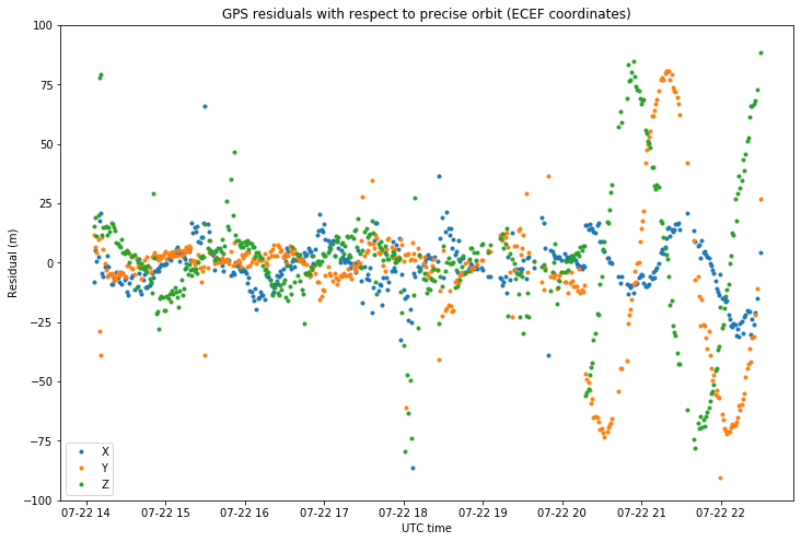
The GMAT script needs to be run first in orbit determination mode to produce the following estimation report. This report is then read in the Jupyter notebook in order to plot the residuals. These are shown below.

For reasons that are explained below, only the first 330 GPS measurements are considered for orbit determination. Therefore, the residuals after 20:00 UTC are much larger.

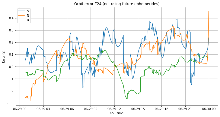
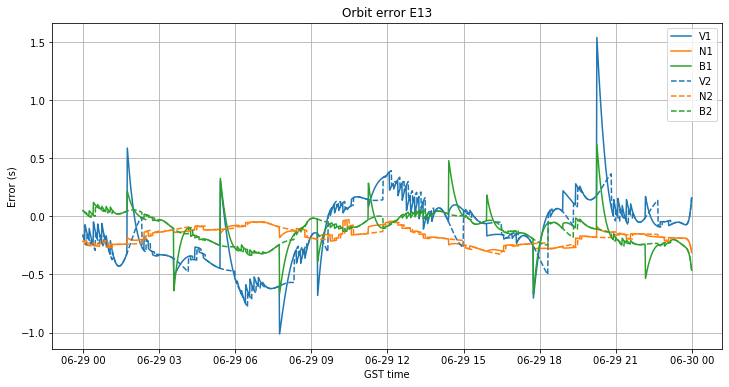
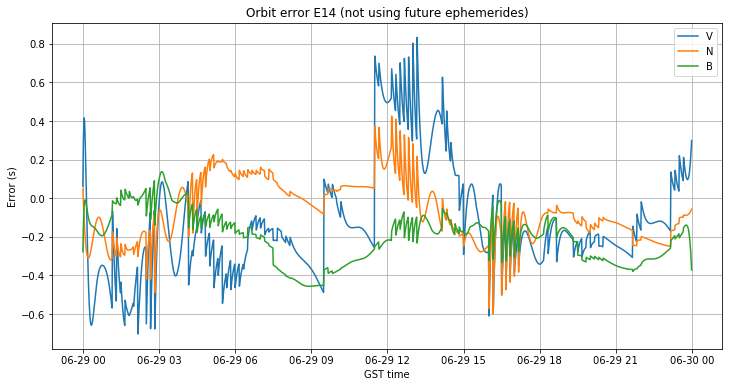
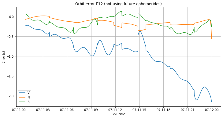
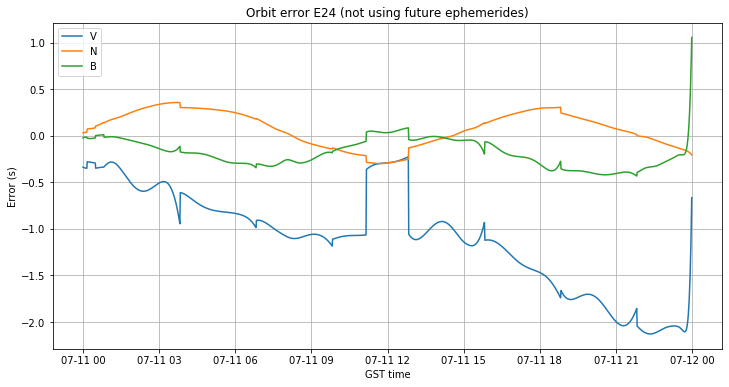
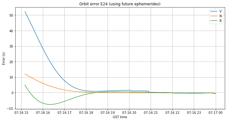
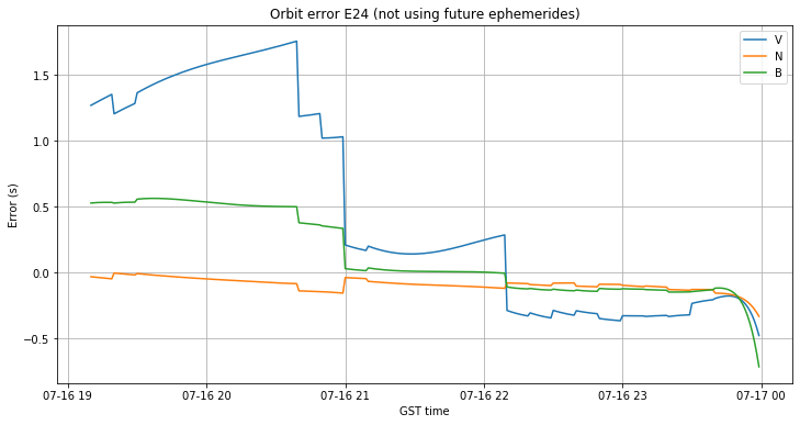
The problem with the plot of residuals shown above is that it is in ECEF coordinates, which are not so easy to interpret. It is much more useful to show the residuals in VNB coordinates, which are formed by a V vector, pointing in the direction of the velocity vector of the spacecraft, an N vector, which is normal to the orbital plane, and a B vector, which completes a right-handed orthonormal frame. The B vector lies in the orbital plane and points towards the Earth (though not exactly towards the Earth centre unless the orbit is circular).

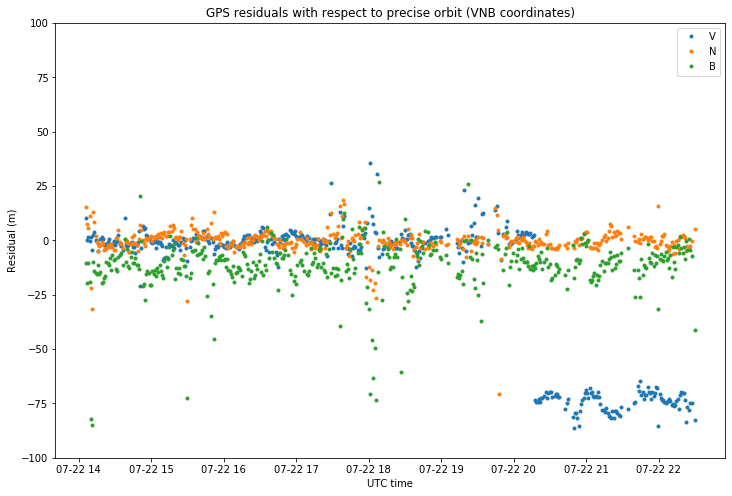
To plot the residuals in VNB coordinates, it is necessary to run the GMAT script again in propagation mode to produce a CCSDS OEM file containing the state vector of Lucky-7 in ECI coordinates. The OEM file is then read in Python, the ECEF residuals are rotated to ECI coordinates using Astropy, and then rotated to VNB coordinates. The results are shown in the figure below.

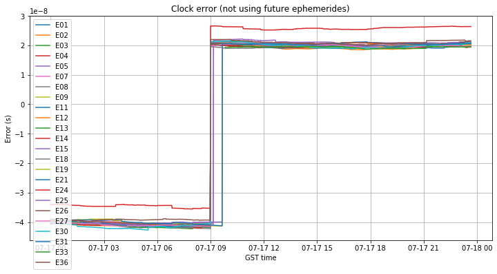
There is a very noticeable jump in the residual of the V coordinate sometime after 20:00 UTC. This is the reason why the measurements after this moment haven’t been included in the orbit determination. The jump is most likely cause by some jump in the clock of the GPS receiver on-board Lucky-7. At an orbital speed of approximately 7.5km/s, 75m corresponds to 10ms. Thus, it seems that at some point the timestamps of the GPS receiver start being 10ms earlier than they should. This is a problem with the GPS receiver. No serious GPS receiver should do this, especially if it is going to be used for orbit determination or other applications where measurement timestamping is critical.

Of course, there is no guarantee that the timestamps for the measurements before 20:00 UTC are correct either. The important point is that all the timestamps need to be consistent, meaning that they have a constant offset to UTC time. The problem here is that this offset jumps at some point.

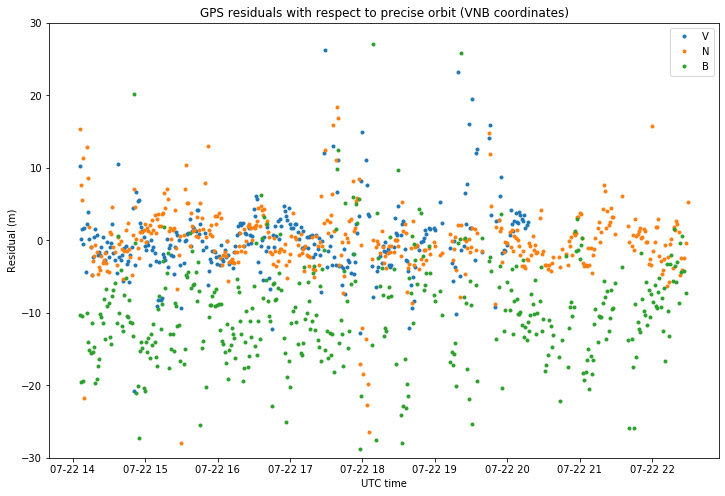
If we zoom in the figure above, we see that the residuals for the V and N coordinates are usually smaller than 5m, which is the typical error that a GPS receiver might give. On the other hand, the residuals for the B coordinate have a much greater standard deviation and seem to be centred on -10m instead of zero.

I am not sure of the reason why the B residuals are biased. The bias means that, according to the GPS measurements, the orbit is 10m higher than the precise orbit found by GMAT. Maybe this is because the drag modelling is not accurate enough.

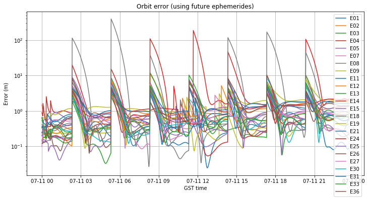
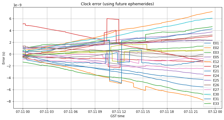
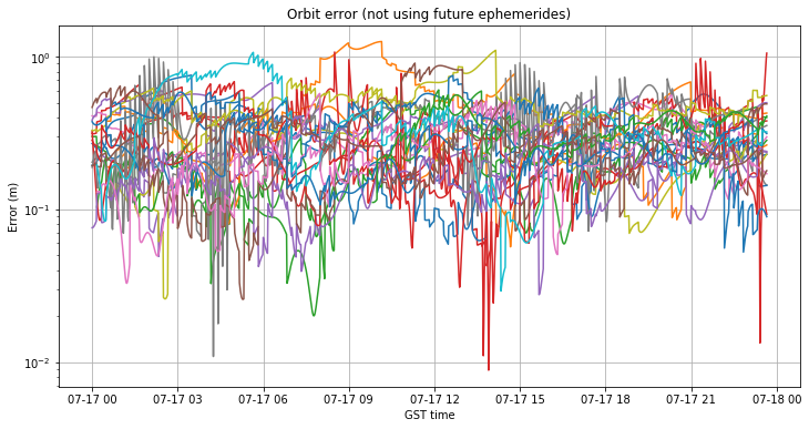
This study has shown the possibilities of running precise orbit determination with a GPS receiver on-board a cubesat in low Earth orbit. For an interval of several revolutions, the orbit is determined with metric level precision. It would be interesting to study measurements over the course of several days to see the magnitude of the effect of orbital perturbations that are not taken into account in the GMAT force model.

Update: After some discussion on Twitter with the SkyFox Labs team, it seems that the problem with the timestamping of the GPS measurements after 20:00 UTC doesn’t have anything to do with the on-board GPS receiver, but rather with the way that the telemetry was processed on ground to produce the CSV file I used. The GPS timestamp is encoded in the Lucky-7 telemetry using 1/256th of a second units (approximately 3.9ms). Then this telemetry was processed with a Scilab script to generate the CSV file.

If we look at the fractional parts of the timestamps in the CSV file, we see that all of them are 0.64 up until some point, where they jump to 0.65. This jump of 10ms coincides with the moment when the jump in the V residual happens.

There is no possible way that the Lucky-7 telemetry has transmitted this jump, as 10ms is not an integer multiple of 1/256 seconds, so this jump must be caused by a bug in the Scilab script.

In fact, correcting the V residuals by adding them the magnitude of the velocity vector times 10ms gives the figure below, where the jump in the V component has disappeared. This shows that all the measurements where taken at a fractional part of 0.64 seconds, despite what the CSV file says.

A couple weeks ago, I did a demo where I showed the LimeRFE radio frequency frontend being used as an HF power amplifier to transmit WSPR in the 10m band. Another demo I wanted to do was to show the LimeNET Micro and LimeRFE as a standalone 2.4GHz transmitter for the QO-100 Amateur radio geostationary satellite.

The LimeNET Micro can be best described as a LimeSDR plus Raspberry Pi, so it can be used as an autonomous transceiver or remotely through an Ethernet network. The LimeRFE has a power amplifier for 2.4GHz. According to the specs, it gives a power of 31dBm, or a bit over 1W. This should be enough to work QO-100 with a typical antenna.

You may have seen the field report article about the QO-100 groundstation I have in my garden. It is based around a LimeSDR Mini and BeagleBone Black single board ARM computer. The groundstation includes a driver amplifier that boosts the LimeSDR to 100mW, and a large power amplifier that gives up to 100W. The LimeSDR Mini and BeagleBone Black give a very similar functionality to the LimeNET Micro, but the LimeNET Micro CPU is more powerful.

The idea for this demo is to replace my QO-100 groundstation by the LimeNET Micro and LimeRFE, maintaining only the antenna, which is a 24dBi WiFi grid parabola, and show how this hardware can be used as a QO-100 groundstation.

For this temporary demo, the hardware is conveniently installed in a hand ladder in front of my QO-100 groundstation weather proof box, as shown in the figure below.

Instead of the usual Airborne 10 low loss coax, I used a smaller diameter coax to connect the LimeRFE to the antenna, since I don’t have an SMA to N female adapter. This coax has somewhat higher losses than the Airborne 10, but it works OK, and indeed I have used it for several months in the groundstation (it can be seen in the field report article images).

The LimeNET Micro and LimeRFE are placed side by side on top of the ladder. The Ethernet cable of the QO-100 groundstation is connected to the LimeNET Micro as a convenient way to access the setup remotely from the house. A GPS antenna is used to lock the LimeNET Micro in frequency. The LimeRFE is controlled by USB from the LimeNET Micro.

Speaking of power supplies, though I have 230VAC in the QO-100 groundstation, this is supplied though a special water tight connector, so it was more convenient to run an extension cord from the house. The LimeNET Micro uses its own 5VDC power supply, while I am using a large 12VDC switched power supply for the LimeRFE.

To simplify things, I have copied where possible the software configuration that I am using in the BeagleBone Black in my QO-100 groundstation. There are two main differences. The first is the PTT control, which in the QO-100 groundstation is done with one of the BeagleBone Black GPIOs, and in the case of the LimeRFE is controlled through a Python script that uses the LimeSuite API, as described in my previous post about the LimeRFE. The second is that, for some reason, the limetx utility from limetool, which is what I normally use to transmit IQ data generated with GNU Radio on my laptop, doesn’t seem to work with the LimeNET Micro. Instead, I have used limesdr_send from limetoolbox, which works well.

For the reception, I am using the same equipment that I use with the QO-100 groundstation: a 120cm offset dish, a GPSDO locked LNB, and a LimeSDR connected to my laptop inside my house. As a GUI for the reception I use Linrad. The IQ samples are received from the LimeSDR using GNU Radio and sent to Linrad with gr-linrad.

Of course it is possible to use the LimeNET Micro in full duplex mode to receive the QO-100 transponder, but I wanted to do a quick demo and concentrate on showcasing the transmit capabilities of the LimeNET Micro and LimeRFE.

After setting up all the hardware and software during this afternoon, I used it for a while on the QO-100 narrow band transponder, demonstrating some of the things I normally do with my groundstation.

First, I put a CW beacon that is generated autonomously in the LimeNET Micro with a Python script that toggles the PTT of the LimeRFE. The LimeNET Micro is generating a continuous carrier with a Python script that transmits a sequence of ones as IQ samples using SoapySDR.

This beacon is really useful to test transmitter power, frequency stability, etc. We see that the frequency stability of the LimeNET Micro is very good, since it is locked to GPS. In this experiment, both the transmitter and receiver are locked to GPS (but using different GPS units).

The power meter is the yellow track on the lower right of the screen. It shows that the signal is 12dB above the noise floor, measured in SSB bandwidth. This is an average power for an SSB station in the QO-100 narrowband transponder. It is amazing how well QO-100 works with only 1W. The digital beacon is usually 18dB above the noise floor, and it marks the maximum power that any station can use. With my QO-100 groundstation I transmit at the beacon level, using around 5W of power.

After this, I demonstrate my GNU Radio SSB transmitter. This runs in my laptop, generating an IQ stream that is sent by TCP to the LimeNET Micro and transmitted using limesdr_send from limetoolbox. Having the GNU Radio transmitter running in my laptop gives me much flexibility as to what modes to transmit (SSB voice, digital, etc.). However, it should be easy to run something similar inside the LimeNET Micro.

First I send a pre-recorded voice and waterfall text CQ. Sending waterfall text is sometimes seen on the narrowband transponder, but it is not very common. I have decided to start using it after seeing Paul Marsh M0EYT use it. I think that it is interesting, because these days most people are looking at a waterfall, so you can see at a glance if any of your friends are on the air calling CQ, without having to listen to a dozen of voice signals. Using a dual waterfall text and voice CQ also takes care of those listening on a conventional radio. My waterfall text has been generated using gr-paint.

After calling CQ for a while, Kurt Moraw DJ0ABR answered. We had a short QSO where I explained him the equipment I was testing and he told me that he uses a 1.2m dish with a 5W homebrew amplifier. In the figure below, you can see one of the overs in the QSO, with Kurt’s signal on the bottom and my signal on the top. Kurt is only 4dB stronger than me.

This demo shows that the LimeNET Micro and LimeRFE is already a complete solution for using the QO-100 narrowband transponder. I think that it is especially interesting for portable stations, if an appropriate box is designed to mount and protect the units. Other interesting projects that are appropriate for the LimeNET are some kind of automated transmitter or transceiver (though be careful when deploying this, as the transponder is a shared and valuable resource), or some sort of signal monitor that searches and analyzes signals in the transponder.

A very interesting possibility that I haven’t explored is to use the LimeNET Micro GPSDO to lock the LNB used for receiving QO-100. There is a clock output connector on the LimeNET Micro, but I think that the frequency of the clock is 30.72MHz. Most PLL-based LNBs need either 25 or 27MHz, so perhaps a PLL to convert the frequency could be used. Alternatively, a good question is if it is possible to do software or hardware modifications to use a 25 or 27MHz clock on the LimeNET Micro.

As you may well know, DSLWP-B, the Chinese lunar orbiting Amateur satellite crashed with the Moon on July 31 as a way to end its mission without leaving debris in orbit. I made a post with my prediction, which showed the impact point southeast of Mare Moscoviense, in the far side of the Moon. Phil Stooke was more precise and located the impact point near the Van Gent crater.

Our plan is to get in contact with the LRO team and try to find the crash site in future LRO images. We are confident that this can be done, since they were able to locate the Beresheet impact site a few months ago. However, to help in the search we need to compute the location of the impact point as accurately as possible, and also come up with some estimate of the error to define a search area where we are likely to find the crash. This post is a detailed account of my calculations.

Digital Elevation Model

So far, all my estimates about the location of the DSLWP-B crash site had used a spherical model for the Moon, simply by asking GMAT to stop the simulation when the spacecraft’s altitude is zero. Phil Stooke recommended us to use a DEM (Digital Elevation Model) of the lunar surface. Since the lunar terrain is quite rough in comparison with Earth’s (changes of several kilometres in terrain height are pretty common all around the lunar surface), the impact site might change noticeably depending on the terrain.

Cees Bassa made a first try at using a DEM a few days ago. His results can be seen in this Jupyter notebook. They show that the impact point is inside the Van Gent X crater, several kilometres away from the location that would have been obtained by assuming a flat surface. This highlights the importance of using a DEM.

The spacecraft track that Cees used for his study is a CSV file published by Wei Mingchuan BG2BHC . The file can be found here. It describes the trajectory of the spacecraft in latitude, longitude and altitude coordinates. The problem with this CSV file is that we are not sure about which hypotheses were used to generate it.

The Moon is much more round than Earth, owing to its low rotational speed. It has an equatorial radius of 1738.1km and a polar radius of 1736.0km. Therefore, for many purposes a spherical model instead of an ellipsoidal model is used. However, there is not a standard lunar radius for the spherical model, and values differing up to 1km are used.

There are two ways of using latitude and longitude coordinates. The first is the geocentric coordinates (called planetocentric coordinates for bodies other than the Earth). These are the well known spherical coordinates. The second is the geodetic coordinates (called planetodetic coordinates for bodies other than the Earth). These use a reference ellipsoid and take into account the ellipsoid flatness, as seen in these formulas. The geocentric coordinates are a special case of geodetic coordinates, where the reference ellipsoid is taken to be a sphere.

For mapping the Earth surface, geodetic coordinates are used almost always. The difference between geodetic and geocentric coordinates is quite noticeable. In the case of the Moon, since its flatness is much smaller than Earth’s, it is common to use planetocentric coordinates instead of planetodetic. The difference between the two coordinates system is smaller than for Earth, but it may still be important for some applications.

The problem with the CSV file generated by Wei is that we don’t know if it uses planetocentric or planetodetic coordinates, nor which is the reference sphere or ellipsoid used to generate the coordinates. Another problem is that we are not sure about the accuracy of the orbital propagation model used to compute the spacecraft’s position in Wei’s file.

In order to have full control over all these parameters, I decided to use GMAT to propagate the orbit and generate the trajectory of the spacecraft in a completely known reference system.

The Digital Elevation Model that Cees is using is SLDEM2015. It is a global model with a resolution of approximately 60m and a vertical accuracy of 3 to 4m. It was generated with data from the Lunar Orbiter Laser Altimeter (LOLA) instrument on-board LRO and the terrain camera on-board the Japanese Kaguya (SELENE) orbiter. More information about this model can be found in this article.

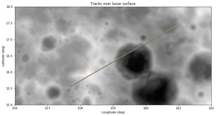
The model can be downloaded here in 30×45 degree tiles. The tile that we use for the DSLWP-B crash site is sldem2015_512_00n_30n_135_180_float.img. Its description can be read here. From this description, it is clear that the file uses a spherical model for the Moon with a radius of 1737.4km. Therefore, the latitude and longitude coordinates used in the DEM are planetocentric.

Additionally, to define the body-fixed coordinate system, the DEM uses the mean Earth/polar axis of DE421, also called MOON_ME. By default, GMAT uses the DE405 solar system ephemeris, but it can be switched to DE421. However, in GMAT, the body-fixed coordinate system of the Moon is defined by the principal axis system, also called MOON_PA. It seems that it should be possible to change this to MOON_ME just by changing the Luna.SpiceFrameId paramter, but the software complains that this parameter cannot be changed in newer versions, and I can confirm that trying to change it makes no effect to the results.

Fortunately, the rotation between MOON_PA and MOON_ME is described by a constant matrix that appears in this document. According to the SPICELunaFrameKernel.tf file in GMAT, the rotation between MOON_PA and MOON_ME in DE421 represents a displacement of 875m on the lunar surface, so the difference is important when computing the DSLWP-B crash site.

In trying to obtain the best compatibility possible with the DEM, I use the DE421 ephemeris in GMAT and output a file with the spacecraft positions in cartesian lunar body-fixed coordinates using the MOON_PA frame. These positions are then rotated to MOON_ME in Python.

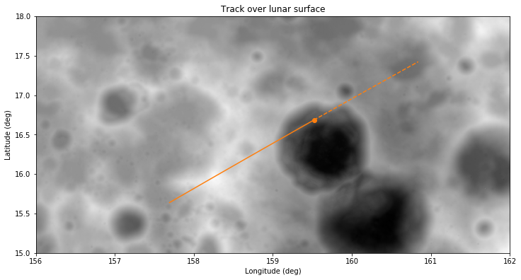
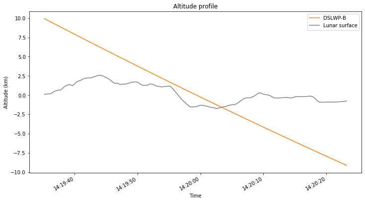
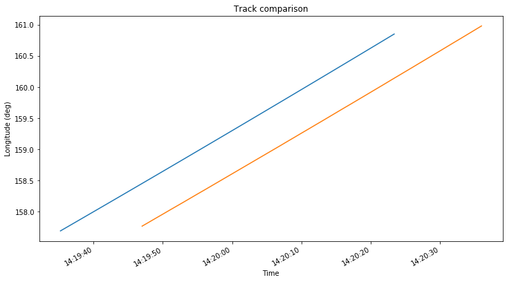
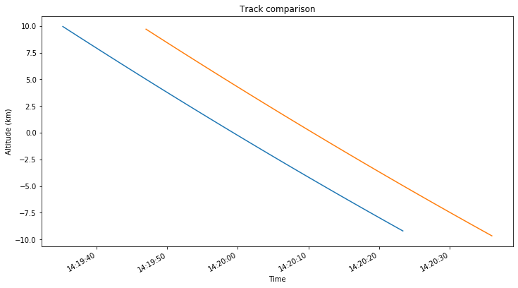
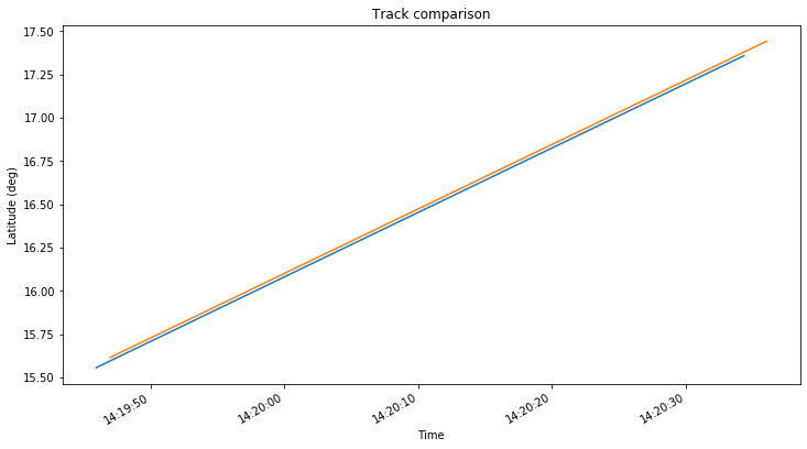
The crash.script GMAT script is used to propagate the spacecraft orbit and the demtrack.py Python file (which is intended to be imported from a Jupyter notebook) is used to load up the DEM, load the GMAT output file, convert from MOON_PA to MOON_ME coordinates, compute latitude, longitude and altitude assuming a lunar radius of 1737.4km, and compute and plot the impact point of the spacecraft’s track with the DEM surface.

The calculations are run from this Jupyter notebook. The figure below shows a track generated with the ephemeris from July 25 that I used in my previous post. DSLWP-B passes approximately 500m above the western rim of Van Gent X crater, enters the crater, and impacts against its northern wall. At a first glance, the results looks close to those obtained by Cees Bassa.

Ephemerides and orbital models

The next step is understanding how much effect do different ephemerides and orbital propagators have on the location of the impact point. This serves to estimate the error of the crash site location prediction and define a search area.

The figures shown above have been done using the ephemeris from July 25 generated by the Chinese DSN. These are the best ephemeris I have so far, since Wei hasn’t been able to find some ephemeris for a later epoch yet.

The force model used in GMAT is rather accurate and it is what I have been using for most of the simulations throughout the mission. It considers the Moon non-spherical gravity using spherical harmonics up to degree and order 10 taken from the LP165P model, the point masses of all the other major bodies in the solar system, solar radiation pressure (although the area and reflectivity coefficients are very rough approximations), and relativistic corrections.

Therefore, in my opinion, the figure shown above represents a good estimate of the impact point, and I will use it as a reference to judge impact points generated using other methods. The coordinates of this reference point are the following:

Latitude 16.6858 deg, Longitude 159.5218 deg, Altitude -1561.12 m

As mentioned above, this assumes a spherical Moon with a radius of 1737.4km and uses the DE421 mean Earth/polar axis reference system.

The first test I have done, to have a coarse estimate of the error of the Chinese DSN ephemerides and the orbital model is to use older ephemerides. The impact point is computed with these older ephemerides and compared with the reference position in East, North, Up (ENU) coordinates. The results are as follows:

Ephemeris from 2019-07-18
East = -64.6 m, North = -221.6 m , Up = -93.1 m

Ephemeris from 2019-06-28
East = 490.5 m, North = -72.6 m , Up = -86.2 m

We see that the error obtained by using older ephemerides is only of several hundreds of metres, even if we use the ephemeris from 2019-06-28, which were taken more than one month before the impact.

Another important task is to compare these results with the CSV file generated by Wei and the results obtained by Cees. Cees gives the coordinates for the impact as latitude 16.675 deg, longitude 159.617deg. In the ENU system centred on my reference point, these are:

East = 2766.3 m, North = -326.9 m

There is a rather noticeable difference of approximately 3km between the result by Cees and the positions I have obtained. If I load up the CSV file made by Wei and study it using my code, I get an impact position of

East = 2752.9 m, North = -311.6 m , Up = -316.0 m

This differs from only in 20m from the position that Cees has obtained. Here we are using the same data for the spacecraft track and DEM, but are doing the calculations independently, using a different algorithm, which explains the difference in positions.

The difference between the positions obtained with Wei’s CSV file and my GMAT simulations is so large that it is worth investigating. The figures below show a comparison of the spacecraft tracks, with my GMAT simulation using the July 25 ephemeris in blue and Wei’s CSV in orange.

It seems that Wei’s track is displaced a few km to the southeast with respect to my track. This makes me suspect about the orbital model used by Wei to generate the CSV.

As a simple test, I run my GMAT simulation using point mass gravity for the Moon. The results are seen below in blue, with Wei’s track in orange. We see that the track generated with spherical gravity in GMAT is much closer to Wei’s track.

The impact point of this GMAT spherical gravity track is given in ENU coordinates as:

East = 3192.5 m, North = -752.4 m , Up = -548.5 m

This is 1150m away from the impact point computed with Wei’s CSV file. Part of this difference may be caused by the difference between the MOON_PA and MOON_ME reference frames. Indeed, if I skip the conversion from MOON_PA to MOON_ME when loading the GMAT spherical gravity track, I get an impact of

East = 3043.6 m, North = -504.8 m , Up = -431.3 m

which is only 870m away from the impact of Wei’s CSV file.

From talking about this problem with Wei, it seems that he is indeed using spherical gravity for the Moon, though I am not completely sure about it. He says he is using STK with the propagator Earth HPOP Default v10.

I think that it is important to use a good non-spherical gravity model for the Moon when computing the impact location, as we have seen that the prediction can change by more than 3km depending on the gravitational model used. Since DSLWP-B’s orbit is elliptical, the non-spherical gravity of the Moon perturbs the orbit noticeably as the satellite passes through the periapsis. Before the crash, the latest periapsis height was only 13km, so non-spherical gravity plays an important role.

Already going to a gravitation model with spherical harmonics of degree up to 2 and order 1 (i.e., considering only the Moon oblateness) gives a similar track to the one with 10×10 spherical harmonics and an impact point of

East = 619.8 m, North = 705.0 m , Up = 152.3 m

Therefore, it seems that most of the effect in the impact point due to the non-spherical gravity is caused by the oblateness term.

To assess whether a 10×10 gravity model is accurate enough for the calculation of the impact point, a simulation with a 20×20 model taken from LP165P has been done using the GMAT ephemeris. This gives an impact point coordinates of

East = 66.8 m, North = 31.8 m , Up = 1.2 m

Since the difference between the 10×10 and 20×20 gravity models is smaller than the error we expect to have in the ephemeris, we conclude that a 10×10 gravity model is appropriate.

Monte Carlo experiments

We do not know the accuracy of the July 25 ephemeris that we are using for the calculations. Often, a state error covariance matrix is used to describe the accuracy, but we don’t have such a matrix. Therefore, Cees suggested to see what would happen if we assumed a position error of 1km in the ephemeris.

To answer Cees’s question, I have run a Monte Carlo simulation where the July 25 ephemeris (in cartesian state) are perturbed using a Gaussian error with a sigma of 1km in position and 0m/s in velocity. The impact point coordinates for each trial are then saved for later analysis. The calculations are done in this Jupyter notebook.

After generating more than 2000 impact points, I plot the results on top of the DEM map, as shown in the figure below.

Most of the impact points are in an ellipsoidal area on the northern wall of Van Gent X. The area is more spread in the direction of DSLWP-B’s orbit, which makes sense. A few of the simulations haven’t managed to clear the western rim of Van Gent X and have impacted on the rim instead.

The points that impact outside of the crater are labeled as outliers and shown in orange in the figure below, which uses ENU coordinates with respect to the reference point given above.

Only 0.6% of the impact points have been classified at outliers, so the probability that DSLWP-B crashed outside of Van Gent X is low.

The covariance of the non-outlier points is then computed in order to give an error ellipse. The eigenvalues of the covariance matrix, which indicate the semi-axes of the ellipse are 876 and 239m. The orientation of the major axis is 57.6º with respect to north.

The figure below shows the non-outlier points with the 1-sigma, 2-sigma, and 3-sigma ellipses.

It is not easy to judge whether the orbital error model of a 1km sigma in position is realistic or not. In my opinion the orbital error should be smaller, and the 1km sigma should be taken as a worst case scenario. Indeed, using the ephemeris of June 28, we obtained an impact point well inside the 1-sigma ellipse of the 1km sigma error model.

Comparison with radio observations

Another idea that Cees suggested to validate the ephemerides was to compare them with radio observations of the Amateur payload done on the days before the crash. One of the things that can be observed are radio occultation timings. According to GMAT with the July 25 ephemeris, the following radio occultations happened before the crash:

2019-07-26 11:31:22.793 --- 2019-07-26 12:15:56.704
2019-07-27 07:53:41.841 --- 2019-07-27 08:35:54.149
2019-07-28 04:17:37.714 --- 2019-07-28 04:56:15.064
2019-07-30 17:38:30.129 --- 2019-07-30 18:07:41.744 (see update)
2019-07-31 14:08:27.941 --- crash

From these occultations, only the ones on July 26 and July 31 were recorded in Dwingeloo. The IQ recordings can be found here.

For July 26, the start of the occultation was observed both in the 435.4MHz and 436.4MHz frequencies at 2651.5 +/- 0.5 seconds since the beginning of the recording. This is a coarse timing for the occultation obtained by looking at the waterfall in inspectrum rather than a precise timing obtained by fitting a diffraction curve.

The end of the occultation was not observed on any of the frequencies. Cees twitted that the occultation ended during a JT4G transmission at 435.4MHz, but as it can be seen in the figure below, the first JT4G tone comes on cleanly rather than being diffracted. This means that the JT4G transmission started shortly after the occultation end.

The recording done on July 26 is timestamped with a start time of 10:47:03 UTC. This is only included in the filename, so I am not completely certain about the accuracy of this timestamp (see below). According to this timestamp, the occultation started at 11:31:14.5 UTC. This is 8.3 seconds before what predicted by the ephemeris.

For July 31, the start of the occultation was observed on both frequencies at 2775 +/- 0.5 seconds after the start of the recording. The recording of July 31 is in GNU Radio metadata format and includes timestamps taken from GPS. The timestamp at the beginning of the file is 2019-07-31 13:22:10.490141 UTC. Thus, the occultation started at 14:08:25.5 UTC. This is 2.4 seconds before what predicted by the ephemeris.

However, the filename says that the recording started at 13:22:02 UTC. Thus, it seems that the filename timestamp is wrong by 8.49 seconds. This perhaps explains the error of 8.3 seconds seen in the July 26 occultation. If we assume that the timestamp in the filename of the recording is 8.5 seconds earlier than the real start of the recording, then it turns out that the July 26 occultation started only 0.2 seconds after what predicted by the ephemeris.

To summarise, we have the following differences between the radio observations of the occultations and the July 25 ephemeris:

July 26:  0.2 +/- 0.5 or 8.3 +/- 0.5 seconds ?? (see update below)
July 31: -2.4 +/- 0.5 seconds

It is not easy to judge the accuracy of the ephemeris from these numbers. First of all, the usefulness of occultation timings is limited, since any difference between the observation and the ephemeris can be explained by a change in mean anomaly, so that the spacecraft travels the same track at a different time, and the change in the impact point location is very small. However, it is worthy to remark that the error in ocultation timings from these ephemeris are an order of magnitude smaller than those observed in my diffraction study, giving more confidence in the accuracy of the July 25 ephemeris.

Cees has also suggested to perform analysis to other parameters of the radio observations, such as the Doppler curve. I am not so sure about the usefulness of Doppler observations. On the one hand there is an unknown transmitter frequency offset, and on the other hand the Doppler usually changes rather slowly, so I am not sure how much can the orbital elements be constrained by Doppler observations.

Update 17:00 UTC: Cees says that he wouldn’t trust transferring the timestamp offset from the tagged recorded to the untagged recording, since these are done in a different computer. He has also noticed that I have forgotten to process two occultations: the one on July 28 (probably because I didn’t see the corresponding recording made at Dwingeloo), and the one on July 30 (because it wasn’t originally listed in the GMAT output, as it happened below 7 degrees of elevation).

I have now processed the occultations on July 28 and July 30. The observation results are as follows:

July 28:
Entry: 04:17:38.3    Exit: 04:56:15.3
July 30:
Entry: 17:38:28.9    Exit: 18:07:41.9

Thus, we obtain the following differences between the observations and GMAT simulation.

July 26 (entry):  0.2 +/- 0.5 or 8.3 +/- 0.5 seconds
July 28 (entry):  0.6 +/- 0.5 seconds
July 28 (exit):   0.2 +/- 0.5 seconds
July 30 (entry): -1.2 +/- 0.5 seconds
July 30 (exit):   0.2 +/- 0.5 seconds
July 31 (entry): -2.4 +/- 0.5 seconds

LRO imaging

According to the calculations above, I expect that the impact point of DSLWP-B should be located near the reference position given by the following planetocentric coordinates in mean Earth/polar axis:

Latitude 16.6858 deg, Longitude 159.5218 deg

I estimate an error of perhaps 600m in the northeast direction and 200m in the southeast direction. This area can be seen here in Quickmap, with the reference point marked (also shown in the figure below for convenience). Fortunately, it seems that the area has few craters, so perhaps it is not difficult to observe any alterations to the terrain.

LRO has three cameras: the wide angle camera (WAC), and two narrow angle cameras (NAC). The NACs have a resolution of 0.5 metres and a swath of 5km. Since LRO is in a polar orbit, NAC images are strips which are 5km wide in the east-west direction and many kilometres long in the north-south direction.

According to the calculations above, it seems enough to take a single NAC image over the reference position in order to have confidence that the real DSLWP-B crash site will appear in the image. To cover a wider area, two or three adjacent NAC images may be taken.

Quickmap can also search for NAC images that contain our reference point. The results are shown here. We see that there are four NAC images available. These can be explored individually, but the interface is not so easy to use as Quickmap, and the east-west directions are swapped. I have taken a look at image M1107231635RC and found that the reference position is around line 8500, sample 3364.

Here I want to show a technique for measuring the gain of a dish that I first learned from an article by Christian Monstein about the Moon’s temperature at a wavelength of 2.77cm. The technique only uses power measurements from an observation of a radio source, at different angles from the boresight. Ideally, the radio source should be strong and point-like. It is also important that the angles at which the power measurements are made are known with good accuracy. This can be achieved either with a good rotator or by letting an astronomical object drift by on a dish that is left stationary.

I will use the Moon noise measurements that I did last month. It is much better to use the Sun instead, which is much stronger. It is also convenient to remark that the Sun and the Moon are not point-like objects, but rather have an apparent radius of around 0.5º. The effects of this will be explained below.

In this post I will be using the notation in the Wikipedia article about antenna gain, where terms such as gain, efficiency and directivity are explained.

When speaking about the gain of a dish, we are really speaking about its directivity. Indeed, if we consider the dish as a transmitting antenna, it is common to assume that all the power radiated by the feed ends up being transmitted somewhere to the far field (even if not in the desired direction). It is reasonable to assume that no power is lost as heat when the radio waves reflect off the dish.

Of course, in a real feed, some power is lost. For instance, Monstein estimates in his article the losses due to the plastic cover in the waveguide of the satellite TV LNB he is using. However, if we are speaking just about the dish itself, it makes sense to assume an lossless feed.

This reasoning justifies that, when considering the gain of a dish, we might take the efficiency of the antenna to be one, so the gain and directivity coincide.

We assume that spherical coordinates \((\theta,\varphi)\) are arranged so that \(\theta \in [0,\pi]\) indicates the angle from the boresight of the dish. Assuming a point-like radio source, the power received when the source is in the direction \((\theta,\varphi)\) is\[P(\theta,\varphi) = \lambda D(\theta,\varphi),\]where \(\lambda\) is a constant and \(D\) denotes the directivity.

By definition of the directivity, we have\[\int_{0}^{2\pi}\int_0^\pi D(\theta,\varphi) \sin \theta\,d\theta d\varphi = \int_{S^2} D(x)\,dA(x) = 4\pi.\]Assuming that the directivity \(D(\theta,\varphi) = D(\theta)\) depends only on \(\theta\), which makes sense, since the radiation pattern of a dish is almost symmetric around the boresight, and that \(D(\theta) = 0\) for \(|\theta| > \theta_0\) for some angle \(\theta_0\), since most of the power radiated by a dish is concentrated in the main lobe of the radiation pattern, then we have\[\int_0^{\theta_0} D(\theta) \sin \theta \, d\theta = 2.\]

This implies that\[\tag{1}\lambda = \frac{1}{2}\int_0^{\theta_0} P(\theta)\sin\theta\,d\theta.\]This integral can be approximated by taking power readings \(P(\theta)\) at different angles from boresight \(\theta\) between 0 and \(\theta_0\). Then the directivity can be computed by dividing the power readings by \(\lambda\), and the gain is simply the directivity in the boresight direction\[G = D(0) = \frac{P(0)}{\lambda}.\]

To perform these calculations, I will use the power readings of Moon noise that I took last month. These can be seen in the graph below.

This data has two main problems. First of all, as I commented in my post about the observation, the pointing of the dish was clearly incorrect. The peak of the noise doesn’t happen when the Moon is closest to the nominal dish pointing. Therefore, I have assumed that the Moon passed through the boresight at the moment when the peak in the noise happened, and derived from that the angle from boresight for each of the measurements.

Of course, it is most likely that the Moon didn’t pass exactly through the boresight, but close to it. The effect of this error is to underestimate the gain, though it is not trivial to see this. The calculations will be shown in a future post.

The second problem is that the Moon noise signal is weak. As remarked above, it is best to use a strong signal. The measurements in the figure above are \(S + N\) (signal plus noise). The power measurements used for the computation of the directivity need to consider only the signal power. For very strong signals, \(S + N \approx S\) is a valid approximation. In other cases, we need to come up with an estimate of \(N\) and subtract that from our measurements. For weak signals, the power measurements of \(S\) are very sensitive to the value chosen for \(N\).

When the signal is far enough from the boresight, it is so weak that it is impossible to estimate \(S\) effectively. Thus, \(P(\theta)\) can only be determined with enough accuracy for small \(\theta\), so we need to set the cutoff \(\theta_0\) small enough so that equation (1) only requires measurements \(P(\theta)\) that we are able to make accurately. This has the effect of overestimating the gain, since by choosing \(\theta_0\) too small, we underestimate \(\lambda\).

Nevertheless, the results that can be obtained with my Moon noise measurement are not so bad. The calculations have been done in this Jupyter notebook. The figure below shows the gain or directivity \(D(\theta)\).

The signal power measurements start being too noisy at around 1.6 degrees from boresight, so the cutoff \(\theta_0\) has been put there. We see that the gain of the 1.2m offset dish at 10366.5MHz is approximately 40.5dBi. The 3dB half beamwidth is approximately 1 degree.

The accuracy of this result is not so bad compared with the theory. In this online dish gain calculator, for a 1.2m dish with an efficiency of 0.65 and a frequency of 10366.5MHz, we get a gain of 40.43dBi and a 3dB half beamwidth of 0.81 degrees.

As we have remarked above, the Moon is not a point source. When the radio source is an extended source, then the power measurements are some sort of convolution between the directivity and the power distribution of the source. This has the effect of smearing out the measured antenna pattern, underestimating the gain, and overestimating the beamwidth. The effects are larger when the radio source is large in comparison with the beamwidth.

More in detail, we assume for simplicity that the source is radially symmetric, with a power distribution \(k(\alpha)\), where \(\alpha\) is the angular distance from the centre of the source, normalized so that\[2\pi \int_0^\pi k(\alpha) \sin \alpha \, d\alpha = 1.\]Note that the left hand side of this equality is\[\int_{S^2} k(\alpha(x,y))\,dA(x),\]where \(y \in S^2\) is arbitrary and \(\alpha(x,y)\) denotes the angular distance between the points \(x\) and \(y\).

For example, the Moon or the Sun may be modeled as a uniform disc of angular radius \(\alpha_0\), so that\[k(\alpha) = \frac{1}{2\pi(1-\cos \alpha_0)},\]for \(\alpha \leq \alpha_0\) and \(k(\alpha) = 0\) elsewhere.

Now, the power reading taken at a point \(x \in S^2\) is\[P(x) = \lambda\int_{S^2} D(y) k(\alpha(x,y))\,dA(y).\]Using Fubini’s theorem, we compute\[\begin{split}\int_{S^2}P(x) dA(x) &= \lambda\int_{S^2}\int_{S^2} D(y)k(\alpha(x,y))\,dA(y)dA(x)\\ &= \lambda\int_{S^2} D(y)\,dA(y) = 4\pi\lambda.\end{split}\]Therefore, equation (1) is still a good approximation for \(\lambda\). However, by dividing \(P(x)\) by \(\lambda\), we are computing the convolution\[\int_{S^2} D(y) k(\alpha(x,y))\,dA(y)\]instead of \(D(x)\). Even in the simple case when \(D\) depends only on \(\theta\) and \(k\) describes the uniform disc model given above, the computation of this convolution is rather involved.

A few weeks ago, a presentation by Octavian Andrei, of the Finnish Geospatial Research Institute, appeared in YouTube showing technical details about the Galileo constellation outage that happened between July 12 and 16. In the presentation, Octavian studies the navigation data gathered by a geodetic receiver in Metsähovi, showing anomalies in some of the parameters of the navigation message, such as the \(\text{IOD}_{\text{nav}}\), the SISA (signal in space accuracy) and the DVS (data validity status).

Back in July, I looked at the navigation data from the outage in this post, where I used navigation RINEX files collected by the IGS MGEX to study changes and anomalies in the navigation message. In that post I concentrated on July 16 and 17, to show what happened as the system was coming back online. Octavian has discovered some very interesting anomalies that happened before the incident, on July 10 and 11. Indeed, the first anomaly happened at 13:40 GST on July 10, well before July 11 21:50 GST, when the navigation message stopped being updated.

Thus, in view of Octavian’s discoveries, I have revisited my study, including also data from July 10 and 11, and paying special attention to the \(\text{IOD}_{\text{nav}}\) parameter, which can be seen to have the most interesting behaviour in Octavian’s presentation.

In my original study, I didn’t pay so much attention to the \(\text{IOD}_{\text{nav}}\) because it behaved rather normally on July 16 and 17. However, since it seems that it plays a key role in how the outage started, I have started by plotting the \(\text{IOD}_{\text{nav}}\) in a very similar manner as to how Octavian does. The figure below shows the evolution of the \(\text{IOD}_{\text{nav}}\) on June 29, which was used as a control day (i.e., a day without anomalies) for my study. We can see the behaviour that Octavian remarks: even thought the \(\text{IOD}_{\text{nav}}\) is a 10 bit number, it increases by one every ten minutes and rolls over after reaching 127.

The figure below shows the \(\text{IOD}_{\text{nav}}\) evolution on July 10 and 11, before the outage happened. All the anomalous details are best seen in Octavian’s video, but here I’ll summarise the most important.

• There is a gap where no updated ephemerides are transmitted shortly after the rollover on July 10.
• At the end of the gap, the \(\text{IOD}_{\text{nav}}\) jumps back up briefly.
• Then it continues updating as if nothing had happened.
• At some point, the ephemeris update rate changes from 10 minutes to 3 hours, and the \(\text{IOD}_{\text{nav}}\) increases a lot with each update.
• This continues until 21:50 GST on July 11, when the last batch is transmitted. Around 12:00 UTC on July 11, some of the satellites transmit batches out of the normal sequence, at an update rate faster than 3 hours.

It is interesting to note that, should the increasing trend of the \(\text{IOD}_{\text{nav}}\) had continued at the same rate every 3 hours, the value would had overflown after 21:50 UTC. Maybe this is just a coincidence, but it might explain why the batch at 21:50 was the last one.

The satellites transmitting anomalous \(\text{IOD}_{\text{nav}}\)’s around 12:00 UTC will be studied in more detail below.

Finally, the figure below shows the evolution of the \(\text{IOD}_{\text{nav}}\) on July 16 and 17, as the system was coming back to normal. Everything looks OK except for a point which doesn’t belong to the normal evolution.

Closer inspection shows that that point correspond to SVN E07, which transmitted an \(\text{IOD}_{\text{nav}}\) of 157 at 20:20 GST on July 17. Below we see that this is the only anomaly. The evolution of the \(\text{IOD}_{\text{nav}}\) of E07 is completely normal if we ignore this unusual jump.

Now we turn our attention to the ephemeris availability during July 10 and 11. The plot, which was first introduced in my study, is show below.

There are two interesting things in this graph. The first is that E21 doesn’t update its navigation message through most of July 10. This is rather unusual and I think no one had noticed it before. The other interesting thing is that we are able to see the satellite that transmit a batch outside of the regular 3 hour pattern. These are E03, E04, E07, E09, E11, E12, E14, E18, E19, E21, E24, E25 and E27. We see that each of these satellites only transmits one or two batches outside of the 3 hour pattern. This is rather interesting, but the reasons for this behaviour are completely unknown to me.

Now we turn to the study of the SISA. Whereas in the previous studies only the values NAPA, 0 (probably a receiver bug) and 3.12m appeared, before the outage we also have the values 3.28m, 3.44m and 3.6m. These are shown in red, purple and brown, respectively. The SISA for the frequency pair E5a,E1 is shown below. The SISA for E5b,E1 behaves very similarly.

The first anomaly in the SISA happens at around 18:00 GST on July 10, when E05 and E08 broadcast 3.6m for a few batches. Then, at around 00:00 GST on July 11 we have all satellites transmitting 3.28m briefly. The 3 hour batches use a SISA of 3.44m. The satellites that break the 3 hour pattern transmit the usual SISA of 3.12m, except for E09, which transmits 3.28m.

The evolution of the DVS is shown below for the E5a signal. The other signals have a very similar behaviour.

The first interesting thing is that satellites E14 and E18 broadcast working without guarantee briefly before 18:00 GST on July 10. These are the eccentric satellites. It seems that Octavian hasn’t consider them in his study. Since they transmit a health status of “in test”, it is possible that the receiver at Metsähovi doesn’t track them.

The second interesting thing is that, after the 3 hour pattern starts, some of the satellites switch to working without guarantee, but not at the same time. These are, the eccentric E14 and E18, which switch on immediately, E11, E12 and E19, which switch at the third batch, and E05, E31 and E33, that switch at the fourth batch.

Gossip is that some satellites have an updated software that detects when the onboard ephemeris expire and sets the DVS to working without guarantee automatically. Presumably, this kind of updates were first installed into the eccentric satellites, due to their unusual orbit. I don’t know how much of this story is true, but it is interesting to note the following: the eccentric satellites switch first, and then all the three IOV satellites E11, E12 and E19. However, there doesn’t seem to be any chronological relation between E05, E31 and E33.

The behaviour of the HS (health status) bits is not very interesting. As usual, the eccentric satellites broadcast “in test”, while the remaining satellites broadcast “OK”.

In summary, this post shows that all the anomalies observed by Octavian can also be seen in the IGS BRDC files. Also, there are some interesting aspects that I haven’t seen that anyone had noticed before:

• E07 transmitting a spurious \(\text{IOD}_{\text{nav}}\) on 2019-07-17 20:20 GST.
• E21 not updating its message during most of 2019-07-10.
• The relation between the SISA and the batches that break the 3 hour pattern.
• The groups of satellites that switched the DVS when the 3 hour pattern started: first the eccentrics, then the IOVs, then E05, E31 and E33.

The plots shown in this post have been made in this Jupyter notebook.

You may have heard about my groundstation for QO-100 (Es’hail-2), which is based on a BeagleBone black and a LimeSDR Mini. A description of this station appeared in a LimeSDR field report. However, I haven’t spoken in detail about the software yet, since I was testing various things and using a makeshift setup until I had some time to put together a solution that I really liked.

Now I am quite happy with the result and indeed I have decided to start up a Github repository with the software I am using in case anyone finds it useful. This post is a description of the software I am using for the narrowband transponder.

The main idea for my narrowband transponder solution is that the BeagleBone Black will just run some software which controls the LimeSDR Mini and streams IQ samples using Ethernet to and from another computer where all the heavy duty work is done. In my case, this computer is my laptop, so I can operate from anywhere in the house, connected through ethernet or even WiFi.

For receiving the downlink, I want to use Linrad because I am a huge fan of that SDR software. I have been using it for all sorts of things, some of which you can see in other blogposts. Thus, it seems natural to use the Linrad network protocol to stream data from the BeagleBone Black. It is also quite nice that this protocol uses multicast UDP, so I can have several instances of Linrad (perhaps on different computers) listening to the same downlink stream.

Since Linrad’s transmit capabilities are not so developed, I am using GNU Radio for the uplink. Most of the time, I will use a GNU Radio flowgraph that gets audio either from my microphone or another application (such as fldigi or WSJT-X) using PulseAudio, filters it to an SSB bandwidth and modulates it on the correct frequency of the transponder. Thus, the GNU Radio flowgraph is essentially an SSB transmiter covering the complete transponder. Using GNU Radio opens up the possibility for other experiments, such as running a digital transmitter implemented completely within GNU Radio.

The main piece of software that runs in the BeagleBone Black is called limesdr_linrad, and is loosely based on the limesdr_toolbox software. It uses the LimeSuite API to drive the LimeSDR Mini in full duplex, streams RX samples using the Linrad network protocol and gets TX samples from a FIFO. The FIFO is then connected to GNU Radio using socat and a TCP stream. I have also tried UDP, but it seems to give some problems with lost packets.

The limesdr_linrad utility implements an additional feature not found in limesdr_toolbox. It can use the LMS7200M NCOs to implement a low-IF instead of the usual zero-IF. This avoids the usual DC spike.

Even though limesdr_linrad accepts parameters to tune to any frequency or use any bandwidth, it is designed with the idea to be used for the QO-100 narrowband transponder in the following manner.

The sample rate is 300ksps, to cover all the 250kHz transponder without wasting network bandwidth. Both the RX and the TX are tuned to the middle of the transponder downlink (in my case a 739.675MHz IF, since I am using a standard Astra LNB with a 9750MHz LO, and 2400.175MHz, since I am modulating directly on 2.4GHz with the LimeSDR Mini).

The RX uses a 0.5MHz low-IF, which is more than enough to avoid the DC spike. The TX uses a 2MHz low-IF. This places the local oscillator at 2398.175MHz, well away from the transponder, in case any LO leakage would get through the transponder. It also helps by filtering out harmonics, since the TX lowpass filter is placed at 3MHz. Of course, the ADCs and DACs of the LMS7200M run at a much higher rate than 300ksps, in order to improve performance, so the LMS7200M FIRs are used for decimation/interpolation, which is what allows us to run the NCOs at a frequency higher than the sample rate. This is all handled behind the scenes by LimeSuite API.

The receive gain is set to 0.2 (normalized gain between 0 and 1 using LMS_SetNormalizedGain()), since there is a short run of coax cable between the LNB and the LimeSDR Mini, so the signal level is already very high. For the transmit gain, I have experimented a little to find the configuration I find most satisfying. This brings me into a discussion of how I like to modulate my SSB voice signal.

The main idea is that I speak normally into the microphone, and the audio gets modulated to RF, without any AGC or compression whatsoever. Compression is used to decrease the PAPR of an SSB voice signal in order to get more power of a PA when the SNR of the signal is not very high. This distorts the voice, but increases the average power, so it is easier to copy the signal in low SNR conditions.

In HF, propagation is unpredictable and we are used to dealing with low SNR signals. Thus, using some form of speech processing to decrease the PAPR is commonplace and helpful. Extreme speech processing is often used in contesting or DX. By boosting some audio frequencies, speech becomes easier to understand in harsh conditions. Unfortunately this has made us get used to all sorts of distorted voice signals.

In contrast, in the QO-100 narrowband transponder the propagation is completely predictable and there is a lot of dynamic range available. The rule is that you should not be stronger than the transponder beacons, but the digital beacon is usually some 18dB (in 2.7kHz of bandwidth) above the transponder noise floor. I have already spoken about the possibilities this gives here, but applied to SSB voice it just means that there is no reason to use speech compression.

Therefore, I just adjust the transmit level so that on voice peaks the average power is approximately at beacon level (where the average power is measured with a reasonable short averaging interval in order to see the power going up and down constantly with the voice articulation). Sometimes the peak envelope power might be well above the beacon level, but if averaged over a whole word, the power I use from the transponder is smaller than that of other stations that use compression.

Since I am using no AGC, there are some precautions and considerations that need to be taken. First of all, the IQ output from the GNU Radio flowgraph should not clip, since clipping would splatter over the whole transponder. This has made me set a rather low gain in the GNU Radio transmitter flowgraph. Most of the time, only a small portion of the LimeSDR Mini DAC full range is used.

On the other hand, since the DAC is run at a reduced range on purpose, the gain of the LimeSDR Mini should be set much higher than in the usual case when DAC is run near full scale. In my case I have no problems with uplink power, because my station includes a 100W PA (intended for the wideband transponder), so I have no concerns about my peak power being limited.

While adjusting the TX gain of the LimeSDR Mini, I have observed that below a normalized gain of 0.62 the TX calibration fails because the TX signal is not strong enough to perform the calibration. The main difference between a successful and an unsuccessful calibration is a huge DC spike (LO leakage) in the case of an unsuccessful calibration. Therefore, it pays off to use a higher gain than desired if this means getting a successful calibration. In this case, the same transmit power can be achieved by using a smaller signal amplitude, and the spurious signals will be much lower. The calibration depends on the gain, so the trick of calibrating at higher gain and then reducing the gain doesn’t really work.

In my case this is not a problem, because for SSB voice I have determined that a normalized gain of around 0.8 is appropriate. If I was going to use only digital signals, which have a much lower PAPR, it would make sense to use the DAC at near full range, and set a much lower range. That would give a gain lower than 0.62 to be at beacon level while running with the DAC near full range. Therefore, it would be better to set the gain at 0.62 and reduce the signal amplitude. In the extreme case where there is a lot of gain in the PA after the LimeSDR and using a gain of 0.62 is absurdly high, an attenuator after the LimeSDR may be used.

Another interesting phenomenon I have encountered in the receive path is that of DC bias. The LMS7200M ADCs have 12 bits. I am using the LMS_FMT_I16 stream format with the LimeSuite API, which puts the 12 bits as the most significant bits of an int16_t. The issue is that the bins of the ADC are not symmetric about zero: the bin corresponding to -1 (-16 when read as an int16_t) has the same probability as the bin corresponding to 0, etc. Therefore, there is a DC bias of -1/2 LSB. It is trivial to correct this by adding 8 to the int16_t samples. If the bias is not corrected, then a DC spike will appear in the middle of the passband, even though a low-IF is being used. Therefore, limesdr_linrad corrects for this bias before streaming the samples to Linrad.

Regarding the Linrad protocol, I have taken most of the implementation from gr-linrad, my GNU Radio out-of-tree module that implements a streamer using the RAW16 and RAW24 Linrad protocols. You can see more information about gr-linrad in this post, including a description of the Linrad network protocol and instructions about how to set up Linrad to receive from the network.

The limesdr_linrad streamer uses the RAW16 protocol. For simplicity, the Linrad TCP server is not implemented within limesdr_linrad, but rather in a Python script called linrad_server.py. This script needs to be run simultaneously to limesdr_linrad.

In the figure below you can see my Linrad setup as I am having a QSO with Wolfgang Knauert DM3AWK.

To receive TX samples from GNU Radio, socat is used. The limesdr_linrad reads samples from a FIFO in /tmp/txfifo to which socat is expected to write. This gives us flexibility in how to interface with GNU Radio and also simplifies the implementation of limesdr_linrad. I am using TCP, so I am running a socat server on the BeagleBone Black by doing

socat -u TCP-LISTEN:6969,fork PIPE:/tmp/txfifo

The GNU Radio flowgraph that I am using to transmit has a simple GUI shown below. The flowgraph gets audio from an Audio source (pulseaudio), modulates it on SSB and sends the samples by TCP.

The spectrum and waveform are shown to help in adjusting the gain. There are fields to enter the gain (or signal amplitude), a frequency correction to compensate the LimeSDR Mini clock drift, and the corresponding downlink frequency of the transmit signal (taking out the 10489MHz part that is common to all the transponder signals). This is done to simplify tuning to the same frequency in Linrad (which also shows downlink frequencies) and the GNU Radio flowgraph. The uplink frequency is shown (without the leading 2400MHz part) for reference when logging the contact.

In my hardware setup, the PA PTT is controlled from a GPIO on the BeagleBone Black. A simple shell script shown below is used to control the PTT easily.

!/bin/sh
 echo $1 > /sys/class/gpio/gpio116/value

Currently I am logging in to the BeagleBone Black with SSH to toggle the PTT. In the future, I will allow the PTT to be controlled directly from the network. Another thing that I want to add to my software setup is Hamlib control, at least to toggle the PTT automatically from digital modes software. I will probably base my Hamlib software on the Python example by Jim Ahlstrom N2ADR.

Another improvement that I want to make to the station is to use an external reference with the LimeSDR Mini. This is probably the first that I will tackle, since it will make operating the station much more comfortable, removing the need to keep adjusting the frequency offset.

Światowid is an Earth observation 2U cubesat built by the Polish company SatRevolution. It carriers a camera with a resolution of 4 metres per pixel and an Amateur radio U/V FM transponder that was never activated due to power budget constraints. The cubesat was launched to the ISS on April 17 this year and released in orbit on July 3. It transmits on the 70cm Amateur satellite band, using 1k2 AFSK AX.25 APRS plaintext for telemetry and 9k6 FSK with a custom protocol for downlinking the camera images. According to the IARU frequency coordination sheet and SatRevolution, it can also transmit images in the 13cm Amateur satellite band at 500kbps.

During June, I worked under a contract with SatRevolution to adapt gr-satellites for their use with Światowid and KRAKsat. Since I am well aware of the problem of private companies using the Amateur satellite bands as “free spectrum” for their satellites, when I was first contacted by SatRevolution regarding this project I did a small background check and saw that Światowid and KRAKsat had obtained an IARU frequency coordination successfully.

I also showed my IARU R1 proposal to SatRevolution and told them that, even though I was signing an NDA for the project, according to ITU regulations they had to publish all the details for the protocols they used on Amateur bands. Formally, these details were not covered by the NDA, and we also agreed that the modified version of gr-satellites would be publicly released under the GPLv3. The decoder was released here on July 4, and this was also announced by SatRevolution on Twitter.

Some Amateurs were not at all happy with the news that the FM transponder was not going to be activated, and accused SatRevolution of adding only the FM transponder to get through the IARU coordination, without having any real intention to activate it, of possibly causing interference to SO-50 and of not giving back anything to the community. However, all of this happened by the time I was already finishing my project with SatRevolution.

After finishing this project, I didn’t merge back to the main version of gr-satellites any of the modifications I did for SatRevolution, and I am not aware of SatRevolution having published any technical information about the 9k6 custom protocol used by Światowid. I didn’t see any reports of people receiving the 9k6 signal (only the APRS telemetry beacon was often seen), so I didn’t consider sorting this out as a priority, since I wasn’t even sure if the 9k6 protocol was actually being used (maybe they were only using S-band to download the images).

A couple days ago, I saw that Piotr Kuligowski SQ4NOW, Maciej Nowak and Tomek SP9TMQ, from the PW-Sat2 team managed to decode one of the images transmitted by Światowid using the 9k6 custom protocol. Talking with Piotr, I learned that they had used my modified gr-satellites version, but as it didn’t provide a complete solution to decode images (below I explain what was missing), they had to do some reverse engineering of the custom protocol.

Now that I’ve learned about the effort of Piotr, Maciej and Tomek, I have decided to add a complete decoder solution for the Światowid 9k6 custom protocol to the main gr-satellites version and to write this post to document completely the protocol.

The Światowid 9k6 protocol is used to transmit JPEG files from the camera. From the point of view of the transmitter, the protocol can be described with these steps:

1. The JPEG file is split into chunks of 48 bytes. The last chunk is padded with zeros at the end in case the file size is not a multiple of 48 bytes.
2. A Reed-Solomon (58, 48) code is used to encode each 48 byte chunk by adding 10 parity check bytes.
3. The 58 byte Reed-Solomon blocks are organized in packets of 141 blocks. The last packet may be shorter if the number of blocks is not a multiple of 141.
4. A CRC-16CCITT zero (see this post about ESEO) of the packet is appended to the packet in big-endian byte format.
5. The length of the packet (including the CRC) in bytes, minus 8, is prepended to the packet as a little-endian 16bit integer.
6. The following data is prepended to the packet, a preamble 0xAAAA, a syncword 0xDADA, and a packet ID 0xBBBB (in this respective order an big-endian format).
7. The packet is sent, with each byte in a least significant bit first fashion, in 9k6 FSK.

I stress that bytes are sent least-significant bit first, which is quite uncommon.

The Reed-Solomon code used corresponds to the following parameters when using Phil Karn KA9Q’s libfec:

• Finite field generator polynomial: 0x11d
• First consecutive root index: 0
• Primitive element index: 1
• Number of roots: 10

This Reed-Solomon code is implemented in many open source libraries which are based in this Wikiversity article, including mersinvald’s Reed-Solomon, Arduino-FEC, and the Python implementation reedsolo, which is what the PW-Sat2 team has used in their reverse engineering effort.

There are a number of drawbacks to the Światowid custom protocol, which make decoding unreliable and likely to fail. First of all, the preamble is very short, making clock recovery difficult for the receiver. Second, the packets are very large. A full packet is 8188 bytes long. This takes 6.8 seconds to transmit at 9k6. Therefore, a lot of data is lost if the packet start is not detected correctly or if a problem such as a clock slip happens mid-packet. The packet length field is not protected by any checksum or FEC, so a bit error in this field will potentially cause a lot of data to be lost as well.

The CRC-16 is somewhat useless, since it is computed on the Reed-Solomon blocks rather than on the data before applying FEC, which is the usual approach. The only way I can think of to use the CRC in this manner is to run Reed-Solomon decoding for each block, recompute the parity check bytes, and check the CRC over this data to see if all the blocks inside the packet were FEC decoded correctly.

The data in each Reed-Solomon block doesn’t have any kind of checksum. Therefore, it is not possible to check if a Reed-Solomon block was decoded without errors. Note that, even though Reed-Solomon is an error correcting code, some blocks at the output of the decoder may still have errors. It is only possible to check if all the 141 blocks inside a packet have been correctly decoded, in the manner remarked above. However, it is not possible to check each block individually.

The packets have no sequence number and there is no indication about the start or end of a file. Therefore, it is difficult or impossible to detect lost packets.

All these problems make it rather difficult to decode an image successfully. For correct decoding, the operator must know where the image starts, maybe by finding the JPEG 0xFFD8FF magic number within the data, and either manage not to lose any packet, or detect packet loss and leave the appropriate gap in the file (although it is difficult to repair a JPEG file with gaps, as some experiments with BY70-1 and other satellites sending images using JPEG instead of SSDV have shown).

There is also a bug in the onboard implementation of this protocol in Światowid, whereby the CRC is omitted from some packets. Presumably this happens whenever a packet doesn’t have 141 Reed-Solomon blocks. Probably it’s possible to detect if a packet is buggy by checking if the length of its payload modulo 58 is either 0 or 2.

The Światowid decoder now available in gr-satellites is not designed to run automatically to reassemble images as other image decoders do, owing to these potential problems in the protocol. It is expected to be run under the supervision of the user, who will then try to reassemble the image manually with the data obtained. It is shown in the figure below.

It works in the following manner. The start of the packet is detected by using 0x5B5BDDDD as a syncword. This is just 0xDADABBBB in least-significant-bit first format. A threshold of zero is used in syncword detection because it is easy to missdetect this syncword, as it has large self-correlation sidelobes.

After detecting the syncword and extracting the 8200 bytes following the syncword, the bytes are reflected to handle the least-significant-bit first format, the packet length is read and the packet is cropped to its correct size. The CRC-16 is checked, but this is only done for informative purposes. The packet is processed regardless of whether the CRC is correct or not.

Each packet is split into FEC blocks and the blocks are then sent to the libfec Reed-Solomon decoder, which prints out whether FEC decoding succeeded or not for each block. The output is then sent into two files. The first, swiatowid_img.jpg, is a concatenation of all the FEC decoded blocks. If the recording processed contains a single image and all the FEC block could be decoded successfully, then this file will contain the JPEG image transmitted by Światowid.

The second file, swiatowid.kss, contains all the decoded FEC blocks in KISS format. This file can be used by an operator that wishes to try to reassemble the JPEG file by hand.

The FEC decoder was not available in the gr-satellites modification I did for SatRevolution, since they intended to do FEC decoding using their own tools, so it wasn’t covered by the contract. Therefore, the PW-Sat2 team have needed to reverse engineer the FEC without any information. Apparently they managed to detect the 58 byte structure somehow.

A sample recording is included in my satellite-recordings repository. This file is an extract from one of the recordings done by the PW-Sat2 team and can be processed by the gr-satellites decoder to yield many correct FEC blocks. However, I haven’t been able to extract the image from the full recording, since none of the FEC blocks in the first packet (which presumably contains the JPEG header) decode successfully. This shows that it is not easy to successfully extract an image from the Światowid signal, making even more remarkable the feat achieved by the PW-Sat2 team.

Yesterday I spoke about the Światowid image downlink protocol. Today, Piotr Kuligowski SQ4NOW has published an image that he has been able to decode from Światowid. The image was taken at around 3:29 UTC and downlinked at 6:38 UTC over Warsaw.

Looking at SatNOGS recordings of this event, I have noticed that the image data is sent with sequence numbers, contrary to what I stated in the description of the protocol in my previous post. This is something that SatRevolution must have added down the road, since it wasn’t present when I worked with them in June.

The protocol is as I described, but the first two bytes of each Reed-Solomon block are used as a little-endian block counter. The remaining 46 bytes are used to send the JPEG file data. The block counter is reset to zero at the start of a new file, and is increased for each Reed-Solomon block.

This block counter allows for automatic detection of lost blocks and start of new images, so I have added an image decoder to the Światowid decoder in gr-satellites. The decoder is based on the 1KUNS-PF image decoder. If there are missing blocks, gaps full of zeros are inserted in the JPEG file in their position. This allows easily merging files decoded from different groundstations just by ORing the files.

As an example showing the image decoder, I have processed this SatNOGS recording, which was made by the station of Cees Bassa in the Netherlands. To process a SatNOGS recording with the gr-satellites decoder, the OGG audio must be converted to WAV (using oggdec, for example), and the gain of the “Multiply Const” block in swiatowid.grc must be changed from 10 to 1, since SatNOGS recordings usually have too much gain.

The recording only contains the beginning of the transmission. The pass was west to east and the transmission was done when the satellite was in view of Warsaw, so by the middle of the transmission the satellite is already below the horizon in the Netherlands. Still, 1128 blocks could be decoded correctly. This amounts to 51888 bytes. The complete file is 204796 bytes long.

The partial image decoded from the SatNOGS recording is shown below.

This image matches the one that Piotr has shown on Twitter. I find it interesting that the SatRevolution logo is already added on-board the satellite to the top left corner of the image.

Last week, the 10GHz beacon ED4YAE on Alto del León was installed again after having been off the air for quite some time (I think a couple of years). The beacon uses a 10MHz OCXO and a 500mW power amplifier, and transmits CW on 10368.862MHz. The message transmitted by the beacon is DE ED4YAE ED4YAE ED4YAE IN70WR30HX, followed by a 5.8 second long tone.

On 2019-08-31, I went to the countryside just outside my city, Tres Cantos, to receive the beacon and do some measurements. The measurements were done around 10:00 UTC from locator IN80DO68TW. The receiving equipment was a 60cm offset dish from diesl.es, an Avenger Ku band LNB, and a LimeSDR USB. Everything was locked to a 10MHz GPSDO. The dish was placed on a camera tripod at a height of approximately 1.5 metres above the ground.

In this post I show the results of my measurements.

The figure below shows my portable setup. Note the GPS magnetic antenna placed on the roof of the car.

The equipment used was a LimeSDR USB, a DF9NP 10MHz GPSDO connected to the LimeSDR and to a DF9NP 27MHz PLL (used to reference the LNB), a LiPo battery, and a laptop computer running Linrad and GNU Radio.

The figure below shows the propagation path from ED4YAE to my station, computed in the SRTM Path Profile software from Mike Willis G0MJW. As you can see, the line of sight path is blocked and the signal refracts on the crest of Sierra de Hoyo de Manzanares midway. This makes it a rather interesting path from the point of view of propagation studies.

Below you can see the view from the top of the dish looking towards ED4YAE. Sierra de Hoyo de Manzanares is visible in the horizon. Behind it, but not visible, is Sierra de Guadarrama, where ED4YAE is located.

Viewing from the LNB, we see more accurately where the dish is pointing. There are two tall white buildings, one of which might be on the way towards the beacon (click on the image to view it in full size).

I recorded the signal of the beacon for several minutes in order to perform measurements later. The first measurement I have done is a frequency measurement. The beacon frequency is 10368861841 +/-5Hz, where the error accounts for the frequency instability. This is only 159Hz lower than the published frequency. It will be interesting to see how the frequency evolves with oscillator aging.

Next, I have studied the propagation path. It can be modeled as a Rician fading channel, with a a strong “line-of-sight” component and several weaker scattered paths. The Rician model depends on two parameters, \(K\), which gives the power ratio between the direct signal and the scattered signals, and \(\Omega\), which gives the total received signal power (including both the direct and scattered signals).

The estimation of the Rician channel parameters has been done separately on each of the beacon long tones by using the Koay inversion technique. The computations have been done in this Jupyter notebook. The figure below shows the evolution of the channel parameters, expressed in dB’s.

We can see that there is some noticeable channel variation over the 12 minutes that the recording spans. The parameter \(K\) changes by up to 8dB, and \(\Omega\) changes by up to 5dB. Even so, the \(K\) is always above 7dB, so the direct signal is predominant.

The next step is to measure the coherence time of the channel. This indicates how fast the channel characteristics change. This is done both in the complex (amplitude and phase) domain and in the amplitude domain.

The first plot shows the normalized self-correlation of the complex baseband signal for each of the measurements (each measurement corresponds to one of the beacon long tones). A loss in self-correlation is mainly caused by a change of phase of 180º, which causes signal cancellation when integrating coherently (note that the frequency of the signal doesn’t affect the self-correlation as long as it is stable).

Except for three anomalous measurements where the coherence time is larger (on one of them it is really large, larger than one second), for most of the measurements the coherence time is between 100 and 200ms. Note that the analysis in the complex domain is affected by frequency instabilities in the receiver and the transmitter, as well as small variations in the propagation delay. To determine whether this coherence time is due to the transmitter and receiver or to the propagation path, the same transmitter and receiver should be measured over a short line-of-sight path.

The next figure shows the normalized self-correlation of the amplitude noise. This means that the amplitude of the signal is taken, the mean is removed, and the self-correlation is computed. In a certain sense, this self-correlation describes how fast the channel fading is changing. For a channel that changes fast, the self-correlation will drop down to zero quickly.

Again, we see coherence times on the order of 100 to 200ms. This analysis in the amplitude domain is not affected by the frequency instabilities of the transmitter and receiver.

We also examine how good is the fit of the Rician model estimated above to the amplitude measurements. The figure below shows the typical case, in which the fit is good.

There are a few measurements where the Rician fit is not so good, such as the one showed below. The plots corresponding to all the measurements can be seen in the Jupyter notebook.

Now we turn to the analysis of the spectrum of the signal. The figure below shows the spectrum of each of the beacon tones. The frequency instability is apparent. There are also some reflections with Dopplers up to 30Hz, which corresponds to 1m/s approximately. The origin of these reflections is unknown.

To compensate for the frequency drift of the signal, it is possible to run the signal through a PLL with a bandwidth of 1Hz and then generate the corresponding spectrum. This is shown below.

The reflections are now more easily visible and it is apparent that they have a decreasing frequency with a similar slope. This is not surprising. A target moving with constant speed on a bistatic radar will always have decreasing Doppler.

There is also a “diffuse haze” that may be caused by transmitter phase noise, by receiver reciprocal mixing, or by the propagation path. Once again, this test should also be done over a short line-of-sight-path to quantify the phase noise effects due to the transmitter and receiver.

The figure below, which shows the spectrum of the beacon tones after being passed by the PLL, shows the characteristics of this “diffuse haze”.

I have spoken about the Galileo incident that occurred in July in several posts already: here I took a look at the navigation message during the outage, here I used MGEX navigation RINEX files to look at the navigation message as the system was recovering, and here I did the same kind of study for the days preceding the outage. Other people, such as the NavSAS group from Politecnico di Torino, and Octavian Andrei from the Finnish Geospatial Research Institute, have made similar studies by looking at the \(\mathrm{IOD}_{\mathrm{nav}}\), data validity and health bits of the navigation message.

However, I haven’t seen any study about the quality of the ephemerides that were broadcast on the days surrounding the outage. The driving force of the studies has been whether the ephemerides were being updated or not, without taking care to check if the ephemerides that were broadcast were any good at all.

The NavSAS group commented seeing position errors of several hundreds of metres during the outage when using the broadcast ephemerides. That is to be expected, as the ephemerides were already many hours old (and indeed many receivers refused to use them, considering them expired). Here I will look at whether the ephemerides were valid (i.e., described the satellite orbit and clock accurately) in their time interval of applicability.

This post is an in-depth look written for a reader with a good GNSS background.

Approach and software used

The main idea of this study is to compare the satellite orbits and clocks computed with the broadcast ephemerides versus the orbits and clocks computed with precise SP3 files. The broadcast ephemerides are obtained from the IGS BRDC broadcast ephemerides navigation RINEX files from IGS MGEX, as in my previous posts. These files are believed to be representative of the navigation message that was broadcast by the satellites. The SP3 files are obtained from the CNES/CLS final solution, which give satellite orbits and clocks at 15 minutes intervals.

It is common understanding that the Galileo outage affected only the ephemerides, and not the navigation signals. Therefore, the SP3 files should be unaffected by the outage, as they are generated from observations of the navigation signals. We are only concerned with detecting large errors in the broadcast ephemerides, such as orbit errors of several metres or clock errors of several nanoseconds. Thus, SP3 files are perfectly accurate for this goal and it is not necessary to use CLK files with high rate satellite clock products. Hence, the SP3 files are taken as a ground truth description of the satellite orbits and clocks.

To compute the satellite orbits and clocks from the RINEX and SP3 files I have used RTKLIB. I am using version 2.4.3 b33, with some additional modifications described later. I have made a simple C program called compute_satpos that uses RTKLIB to load a RINEX and SP3 file, and computes the orbit and clock of each of the Galileo satellites at one minute spacing using both the broadcast ephemerides from the RINEX and the SP3 file. The results are stored in a binary file that can be read later in a Jupyter notebook for plotting and analysis.

Antenna phase centre versus satellite centre of mass

There is an important technical detail regarding the comparison of broadcast ephemerides and SP3 files. The broadcast ephemerides describe the position of the antenna phase centre, while the SP3 files describe the position of the centre of mass of the satellite. To compare both it is necessary to know the offset of the antenna phase centre with respect to the centre of mass, and the attitude of the satellite. The offset is usually stored in an ANTEX file.

The ANTEX file convention uses a simple model for the satellite attitude that allows to define a satellite-fixed frame of reference in the following way:

• The z-axis points toward the geocenter
• The y-axis (rotation axis of the solar panels) corresponds to the cross product of the z-axis with the vector from the satellite to the Sun
• The x-axis completes the right-handed system

The vector from the centre of mass to the antenna phase centre is described using this frame of reference. Therefore, knowledge of the satellite and Sun positions in ECEF coordinates, together with the information in the ANTEX file, are enough to compute the vector joining the centre of mass and the antenna phase centre in ECEF coordinates.

RTKLIB has the function satantoff() to compute the offset using this algorithm and the information loaded up from an ANTEX file using the function readpcv(). The function satantoff() is automatically called when computing the satellite orbit and clock using satpos(), so that as long as an appropriate ANTEX has been loaded, the antenna phase centre instead of the centre of mass is returned.

The problem is that Galileo has a more sophisticated way of dealing with the offset between the antenna phase centre and the satellite centre of mass. The approach is described in the Galileo Satellite Metadata webpage.

First, a reference frame is defined for the satellite. The axes of this frame correspond to the axes used by the ANTEX file (except for a change of signs in the x- and y- axes), but the origin of the frame is a well defined physical point in the satellite rather than the satellite centre of mass. The motivation for the definition of the reference frame is that the reference frame is fixed with respect to the satellite body, while the position of the centre of mass will change as fuel gets used. By defining the positions of the objects in the satellite body with respect to the reference frame rather than the centre of mass, we get coordinates that don’t change as fuel is spent. To complicate matters further, the reference frame is different for the IOV and for the FOC satellites, since the structure of the satellite body is quite different.

The current and historical positions of the centres of mass of the satellites, measured in the satellite reference frame, can be found in the International Laser Ranging service, as well as in the Galileo Satellite Metadata page.

In order to define the antenna phase centre position, first an antenna reference point is defined. This is a well defined physical point located close to the antenna groundplane, so that its position with respect to the reference frame can be measured physically and will not change. The location of the antenna reference point with respect to the reference frame for each satellite is given in the Satellite Metadata. All the IOV satellites have the same location, and all the FOC satellites have the same location, since these only depend on the physical structure of the satellite.

For convenience, the antenna reference point position is also listed “with respect to ANTEX reference frame”, which means the offset from the centre of mass in the ANTEX xyz frame described above. Note that these offsets will change as fuel is spent.

Finally, the antenna phase centre offset is the vector from the antenna reference point to the antenna phase centre. This is given both in the “mechanical reference frame” and in the “ANTEX reference frame”, but the only difference is the sign of the x- and y- axes, since the origin of the offset is always the antenna phase centre.

An ANTEX file is provided in the Galileo Satellite Metadata page. It gives antenna phase centres and phase centre variations (direction-dependant corrections). However, the ANTEX file is described with respect to the antenna reference point and not to the centre of mass, as expected by the ANTEX file convention. Therefore, RTKLIB won’t work correctly with this ANTEX file.

Another important ingredient to compute the offset between the antenna phase centre and the centre of mass in ECEF coordinates is the attitude of the satellite. As introduced in the ANTEX file convention, one axis of the spacecraft body always points to the geocenter, so that the antenna boresight points to the Earth surface. The spacecraft is then free to rotate around this axis. How it rotates is referred to as yaw steering law. Since the spacecraft needs to orient its solar panels orthogonal to the solar rays, the yaw steering law often dictates that the axis of rotation of the solar panels should be orthogonal to the vector joining the satellite and the Sun, as described in the ANTEX file convention. This is the yaw steering law that is implemented in RTKLIB.

The Galileo Satellite Metadata webpage describes in detail the yaw steering laws of the satellites, in a seemingly different way for the IOV and FOC spacecrafts. Upon closer inspection, it turns out that the yaw steering law for the IOV and FOC satellites is only different in the degenerate case, when the sun angle \(\beta\) (the angle between the orbital plane and the solar rays) is small. In this case special case, the nominal yaw steering law described in the ANTEX file convention is not followed, as it would imply very fast yaw changes. The steering law under these uncommon circumstances is different from the ANTEX file convention, but the rest of the time both the IOV and FOC satellites follow the nominal steering law.

Therefore, we need not worry much about the steering law. The nominal law implemented in RTKLIB is valid for the Galileo satellites in most cases. However, we need an ANTEX file in a suitable format which lists the offsets between the centre of mass and antenna phase centre, rather than the offsets between the antenna reference point and the antenna phase centre, as the Galileo ANTEX file does.

To this end, I have modified the Galileo ANTEX file by using the information in the Galileo Satellite Metadata webpage. To compute the vector joining the centre of mass and the antenna phase centre, it is enough to add the vector listed as “ARP in ANTEX RF” and the vector listed as “PCO in ANTEX RF”. The resulting ANTEX file can be obtained here.

Using this ANTEX file, RTKLIB can compute the antenna phase centre when using an SP3 file, allowing the comparison of broadcast ephemerides and precise SP3 ephemerides.

As an example, the figure below shows the broadcast ephemeris orbit error (i.e., the difference between the orbit computed with the broadcast ephemerides and with the SP3 file) of the satellite E24 in VNB coordinates. The VNB (velocity-normal-binormal) reference frame, which is common in the study of orbital mechanics, was defined in my Lucky-7 precise orbit determination post, and the code for computing this frame is taken from there.

We see that the error in each of the components is smaller than 30cm. Since the offset in the z-axis between the centre of mass and the antenna phase centre is usually between 60 and 80cm (63cm for E24), not correcting for the antenna phase centre offset would cause an error of 60 to 80cm in the binormal component (since the z-axis is almost aligned with the binormal axis, as the orbit is almost circular).

As a final note, no care has been taken in RTKLIB regarding the selection of the frequency band (or bands) for the computation of the antenna phase centre position. Depending on the frequency band, the antenna phase centre offset can change by more than 10cm. The ANTEX file describes the offset for each of the bands E1, E5a, E5b, E6 and E5 (AltBOC). When using an SP3 file with a code or carrier observation in one of these bands, the appropriate antenna phase centre should be computed. If the observation is a linear combination of observations on different bands (for instance, an iononsphere-free combination) it is common to take as phase centre a weighted average of the corresponding antenna phase centres (see the RTKLIB implementation).

When using the broadcast ephemerides, one needs to keep in mind that the I/NAV ephemerides are intended to be used with either E5b, with E1, or with the ionosphere-free combination of E5b and E1, and the F/NAV ephemerides are intended to be used either with E5a, with E1, or with the ionosphere-free combination of E5a and E1. However, the orbit parameters transmitted in the I/NAV and F/NAV ephemerides are the same (or almost the same), so with the broadcast ephemeris model the antenna phase centre position is considered to be the same for all bands. In contrast, the clock \(a_{f0}\) parameters are different in the I/NAV and F/NAV parameters and must be corrected with the appropriate BGD if a single band observation is used, since the difference between the group delays on each band is much larger (something on the order of 50ns, or 15m) than the difference in the phase centre positions.

Interval of applicability of ephemerides

A rather striking fact that I’ve discovered when comparing broadcast ephemeris with precise SP3 files is that it is very important to take into account the interval in which each ephemeris is applicable, understood as the interval in which the error doesn’t grow too large.

It is commonly thought that ephemeris describe an approximation of the orbit about the \(t_{0e}\) timestamp, and they are good for a few hours (4 hours is usually quoted) about this \(t_{0e}\). Therefore, when selecting the best ephemeris to use for a particular timestamp, the one with the nearest \(t_{0e}\) is selected, unless the difference in timestamps is larger than a few hours, in which case it is considered that there is no valid ephemeris for that timestamp. This is what RTKLIB does, as one can see in the function seleph().

However, this is not completely true, and unexpected problems can appear when using this approach. Let us see an example. In my previous posts about the outage, I used the broadcast ephemerides from 2019-06-29, which was an uneventful day for the Galileo constellation, as some sort of control to check that both my algorithms and the data were correct and no unexpected effects showed up. The figure below shows the orbit error of the broadcast ephemerides for each of the satellites in the constellation during this day.

As we see, E14 and E18, which are the eccentric satellites have errors which sometimes spike up to more than 10m. This is quite large. Upon further inspection we see that the error is largest just after RTKLIB has made a change in the choice of ephemeris. This happens at the midpoint of the \(t_{0e}\)’s of each consecutive pair of ephemerides.

It turns out that Galileo ephemeris are always started to be broadcast by the satellites after their corresponding \(t_{0e}\). I haven’t seen this written in any of the documents, but it is what happens in practice. A look at galmon.eu, a webpage that shows the latest navigation messages transmitted by the GNSS satellites and marks any possible anomaly, reveals that the Galileo ephemeris age is always shown as “x minutes ago”. The same happens for Beidou and GLONASS, so it seems that all these systems start broadcasting the ephemerides after their \(t_{0e}\). In contrast, GPS often shows an age of “in x minutes”, which means that the ephemerides are started to be broadcast before their \(t_{0e}\).

This is important, because a receiver working in real time with the broadcast ephemeris will never use ephemerides which haven’t been broadcast yet. In the case of Galileo, this means that it will never use ephemerides with a \(t_{0e}\) in the future. Therefore, such a receiver will not see the large errors that appear in the figure above.

Indeed, I have modified RTKLIB to prevent it from choosing ephemerides with a \(t_{0e}\) in the future. The modified version can be found in my nofutureeph RTKLIB branch. The resulting error with this modified choice of ephemerides is shown below.

The result is strikingly much better than in the case when future ephemerides where chosen. Now the orbit error never exceeds 1m, even for the eccentric satellites E14 and E18. I stress that this goes against the common belief that the choice of ephemeris is not very important as long as the \(t_{0e}\) is not very far off, and that when in doubt one should choose the ephemeris with nearest \(t_{0e}\).

This example teaches a good lesson, but I think it is important to reflect on the matter further. The only official information about when Galileo broadcast ephemeris should or should not be used is the answers to the public consultation about the OS ICD. This document used to be accessible until a couple days ago (indeed I’ve already referenced it in some of my older posts), but now it seems that it’s not available anymore.

According to thas document, a receiver should always use the latest ephemerides that have been broadcast. If no new ephemeris are broadcast, the ephemerides can be used for up to 3 hours after their \(t_{0e}\). But the moment newer ephemerides are broadcast, the old ones are considered expired and should not be used even if less than 3 hours have passed since their \(t_{0e}\).

Thus, I think it is useful to introduce the concept of ephemeris broadcast lifetime. This is the time interval when a particular ephemeris is being broadcast by the satellites. In these terms, the Galileo rules of ephemeris use can be expressed by saying that ephemeris can only be used inside their broadcast lifetime and never more than 3 hours after their \(t_{0e}\).

This raises the natural question of what is the broadcast lifetime, or more precisely, what is the broadcast lifetime in relation to the \(t_{0e}\). We have hinted at this question above when we commented that the broadcast lifetime for Galileo, Beidou and GLONASS seems to start after the \(t_{0e}\), while the broadcast lifetime for GPS seems to start before the \(t_{0e}\).

A comparison between the “transmission time of message” and \(t_{0e}\) fields in the navigation RINEX files show that most of Galileo ephemeris in the RINEX files have been received 740 seconds later than their \(t_{0e}\). Other ephemeris show values larger than 740 seconds, but there is none which was received earlier than this. This seems to indicate that the Galileo ephemeris broadcast lifetime starts 740 seconds (12 minutes and 20 seconds) after the \(t_{0e}\). I haven’t seen this value indicated anywhere in the documentation. This is also surprising, considering that often ephemeris are updated every 10 minutes.

By now it is clear that the ephemerides are designed to be used only during their broadcast lifetime. This is illustrated by the example above. The case in which we don’t use future ephemeris doesn’t completely follow the broadcast lifetime rules (as it starts to use an ephemeris at its \(t_{0e}\) rather than 740 seconds after the \(t_{0e}\)), but gives good results. In contrast, the case in which we use future ephemeris shows the problems that can arise whenever ephemeris are used several tens of minutes away from their broadcast lifetime (more on this will appear in the sequel).

Once that it is clear what is the intended applicability interval for the ephemerides, the natural question is what is the real applicability interval. In other words, how much away from the broadcast lifetime can we use the ephemerides without obtaining a too large error. Another important question is why, meaning what makes the error grow relatively quick outside of the broadcast lifetime to the point that ephemerides are no longer usable.

Again, this is best illustrated with a particular example taken from the control day. The figure below shows the orbit error in VNB coordinates for the satellite E13 (a rather uninteresting and normal satellite) both using the choice of future ephemerides (solid lines) and avoiding the choice of future ephemerides (dashed lines).

We see that even though the error doesn’t grow to 10m as it happened with the eccentric satellites when we chose future ephemerides, still there are some large spikes that correspond to the future ephemerides. Half of the time the solid and dashed lines coincide, since both are using the same ephemerides. The remaining half of the time they don’t coincide, because the solid line has already changed to the next ephemeris while the dashed line still maintains the old ephemeris. By changing later, the dashed line avoids the large errors.

If we reflect upon this, we can see that there is something that is perhaps not very reasonable. The error grows rather quickly. In the figure above, in some 30 minutes it grows to more than 1 metre. I don’t think that the error in GPS grows as quickly, since often the GPS ephemerides are used more than 1 hour away from their \(t_{0e}\), and the error obtained when doing so is not several metres.

I think it is interesting to look at the moments in the figure above when ephemerides are being refreshed every 10 minutes. These parts look like a zigzag line in the graph due to the frequent changes between different ephemeris. Now, the orbit error might be quite small, but the derivative of the error is large. Only by jumping to a new ephemeris (and producing a discontinuity) the error is maintained small. However, if we use one of these ephemeris one hour away from their \(t_{0e}\), we find that the error has grown very quickly.

This effect is best seen in the figure below, which shows the orbit error for the eccentric satellite E14 when not using future ephemerides. We see that the derivative of the error is very large at the moments when the ephemerides are changed every 10 minutes. Only by jumping to new ephemeris the error is kept small. If we propagate one of these ephemerides much longer than 10 minutes, we get a very large error, which is what happened when using future ephemerides.

This also seems to explains why ephemerides are sometimes changed every 10 minutes and sometimes not, which was a question in one of my previous posts. The change every 10 minutes is only done when it is necessary to keep the error small because of the error derivative being large. When the derivative of the error is small, such as around 09:00 in the figure above, the same ephemeris can be maintained for more than an hour, since no change is needed to keep the error small.

And now the question is why is the error derivative so large sometimes. Recall that a Keplerian orbit depends on 6 parameters, so to each spacecraft state vector (position and velocity vectors) there corresponds a unique Keplerian orbit that can be considered as the osculating orbit. This is the orbit that the spacecraft would follow if the only force acting upon it was the spherical gravitational force of the central body.

The broadcast ephemerides are based on the Keplerian orbit but include additional perturbations to give a more accurate approximation to the real orbit. These are \(\Delta n\) (a perturbation of mean motion), \(\dot{\Omega}\) and \(\dot{i}\) (the time derivatives of the RAAN and inclination), and harmonic corrections to the anomaly, inclination and orbit radius. Therefore, the broadcast ephemeris model can be considered overdetermined. While for each time there is a single Keplerian orbit that is osculating to the real orbit at that time, the broadcast ephemeris model has many additional perturbation parameters that can be used to obtain a better fit over a time interval. There is much freedom in how to choose these parameters to obtain good results.

I am suspicious that there is perhaps a problem of overfitting with the Galileo ephemerides. By trying to compute the parameters that give the best fit in a certain time interval (probably the broadcast lifetime interval), the model obtained could give a rather poor fit outside of that interval. This is a well known phenomenon that appears in approximation theory. For example, if we try to approximate a continuous function by a polynomial uniformly in some interval, such polynomial will often give a poor fit outside of that interval.

So if I had to guess, I would say that, by trying to improve the broadcast ephemeris fit in some particular interval, too large perturbations to the Keplerian model are chosen. These give a good fit inside said interval, but the error grows quickly, so the fit outside the interval is poor. However, this is probably a topic for a future post.

Control day: 2019-06-29

First we look at the ephemeris error during the control day, June 29, which I chose as an uneventful day for the Galileo constellation. The figures below show the broadcast ephemeris orbit and clock errors when allowing RTKLIB to choose future ephemerides (this has been treated in the previous section). Only the satellites that exceed some predefined error are identified in the legend.

As we have remarked in the previous section, the orbit error stays under 1m except for the eccentric satellites E14 and E18. The clock error of all the satellites is well bounded between -2 and 2 ns, except for E24, which shows a clock error around 6ns. I don’t know what is the cause of this discrepancy, but it is present in all the other days I have analyzed.

If we do not allow RTKLIB to choose future ephemerides, we get the results shown in the figures below.

The orbit error has now improved significantly. It is under 1m for all satellites, and usually around 20 to 30cm. The clock error behaves very similarly independently of whether future ephemeris are used or not.

Following the reasoning about the ephemeris broadcast life described in the previous section, the case when future ephemerides are not used will be taken as representative of the broadcast ephemeris quality in all the scenarios.

Now that we know what errors to expect from the broadcast ephemerides during a regular day, we can pass to study the scenarios corresponding to the days before and after the outage.

Day before the outage: 2019-07-10

The behaviour of the navigation message on the two days before the outage can be found in this post. The figure below, taken from that post, summarizes the evolution of the \(\mathrm{IOD}_{\mathrm{nav}}\).

We see that on July 10 there is a long gap in the broadcast ephemerides between approximately 13:40 and 16:40 GST. Ephemerides are broadcast again at 16:40, but after this there are no ephemerides until 17:30.

The figures below show the orbit and clock errors when future ephemerides are not used. The gap between 13:40 and 16:40 is apparent. The eccentric satellites E14 and E18 quickly pick up very large orbit errors: more than 10m and 100m respectively. In comparison, the other satellites stay with errors below 1m.

The clock error diverges linearly during the gap. This behaviour is to be expected, since the broadcast ephemeris clock model is usually a linear function (a quadratic function is also supported) but the estimation of the slope \(a_{f1}\) will never be perfect. The divergence is small, so only E02 and E19 exceed 2.5ns of clock error. However, it is interesting that with the ephemerides of 16:40 the clock error isn’t corrected and keeps growing. I believe that this is caused by a problem with the determination of the satellite clocks by the ground segment. This will be more clear with the analysis of the next day.

If we plot the orbit error of E14, we see that even though the last set of ephemerides before the gap was at 13:40, the error stays reasonably small until 15:00. Sometime after 15:00 the error grows up very quickly in all the components of the VNB frame. This shows the problems remarked above about the interval of applicability of the broadcast ephemerides, which often seems too small, causing problems like this when no updated ephemerides are broadcast.

If we allow RTKLIB to use future ephemerides, we get the orbit and clock errors shown in the figures below. This time all the satellites get large orbit errors at 15:10, often reaching up to 8m. The reason is that RTKLIB is using the ephemerides from 16:40 rather than those from 13:40. This gives a good example of why the usual rule of choosing the broadcast ephemerides with nearest \(t_{0e}\) may not be a good idea for Galileo. Propagating ephemerides backwards gives larger errors than propagating forwards.

For an more detailed example of this effect, the figure below shows the orbit error of E24 with future ephemerides (solid line) and no future ephemerides (dashed line). We see that between 15:10 and 16:00, when using the future ephemerides, the ephemeris from 16:40 is chosen, causing a large error. In contrast, when using no future ephemerides, the ephemeris from 13:40 is chosen and the error is kept small. I think this kind of examples support my idea that Galileo ephemerides are overfitted in a certain sense.

In summary, on July 10 there was a 3 hour gap in ephemerides between 13:40 and 16:40. The impact to the system performance was small but noticeable for the non-eccentric satellites and receivers using the broadcast lifetime rule. However, there was a large degradation in performance for the eccentric satellites and for postprocessing using the ephemerides with nearest \(t_{0e}\).

Outage day: 2019-07-11

In July 11 there were a few sets of ephemerides broadcast at the beginning of the day, but at 00:50 the broadcast changed to every 3 hours, except for some satellites that transmitted a few ephemerides outside of this schedule (see more details in the previous post).

The orbit and clock errors not using future ephemerides are shown in the two figures below. Regarding the orbit error, we see the same problems on the eccentric E14 and E18 as on July 10, caused by the large 3 hours gaps in the ephemerides. We also note a slow but noticeable tendency of the orbit error of all the other satellites to increase throughout the day. By the end of the day, E12, E19 and E24 already have picked up more than 2m of orbit error.

Regarding the clock error, we see that it grows linearly for all the satellites. There are some strange jumps around 12:00. These seem to correspond to satellites transmitting out of the 3 hour schedule, since there is always a first jump that is not aligned with the 3 hour schedule and only happens for a single satellite, and then a second jump coincident with the 3 hour schedule, where all the satellites that jumped go back to the previous clock error trend. I have no clue about what could cause these jumps, but they are certainly interesting.

Other than the jumps, it seems that the clock model is not being updated regardless of the fact that new ephemerides are broadcast every 3 hours. It seems that the determination of satellite clocks by the ground segment was not working at all. By the end of the day some of the satellites have already picked up to 8ns (or 2.4m) of clock error.

The figure below shows the orbit error of E12 in VNB coordinates. This was one of the satellites whose error grew largest. We see that the error grows mostly in the V component. This is usual in orbital mechanics. Every inaccuracy in the orbit model manifests much more in the V component, since errors such as an error in mean motion build up with time, causing an increasing error in mean anomaly.

Below we show the orbit error of E24, which is one of the satellites whose clock jumped. There is a jump in the orbit and it is aligned with the clock jump. We also see the error buildup in the V component.

Finally, we show the orbit and clock errors when RTKLIB is allowed to choose future ephemerides. The characteristic problem with using future ephemerides happens now for all the satellites every 3 hours, causing orbit errors of several metres.

In summary, on July 11 the performance of the system was degraded even for receivers using non-eccentric satellites and the broadcast lifetime rule. By the end of the day, many satellites had grown orbit errors near 1m and clock errors near 5ns. It seems that the clock model of the satellites wasn’t updated throughout the day, letting the clock error grow linearly.

First day of recovery: 2019-07-16

On July 16, most of the satellites started broadcasting updated ephemerides again at 18:50, after having been several days broadcasting the same old set of ephemerides. The remaining satellites joined a few hours later. More details can be seen in this post.

The figures below show the orbit and clock errors when future ephemerides are not used. The orbit error is smaller than 1m for most of the satellites, and perhaps it seems to improve somewhat during the course of the day.

The clock error seems also well controlled, but in comparison to the control day 2019-06-29, it seems that the clock errors of all the satellites are shifted down around 2ns.

If we let RTKLIB use future ephemerides, it propagates backwards the ephemerides from 18:50 until 14:50. We see that the orbit error grows almost exponentially with time. At three hours of propagation the error is around 10m for most of the satellites, and 100m for the eccentric satellites. At four hours, the error is between 50 and 100m for most of the satellites, and the eccentric satellites reach 1km of error. This shows that, in general, the Galileo broadcast ephemerides cannot be propagated for 3 or 4 hours.

On the other hand, the clock error grows linearly but slowly when propagating the ephemerides backwards. After 4 hours of propagation, the error has perhaps grown 0.25ns, which is completely acceptable.

The figure below shows the growth of the orbit error when propagating backwards the ephemeris of E24. The error grows mainly in the V component, but the error in N and B is also large.

If we don’t allow RTKLIB to use future ephemerides, we get the orbit error shown below instead. It seems that the orbit of E24 was refined during the course of the day. The V error started large and with an increasing trend, but dropped down significantly at 21:00.

In summary, once that updated ephemerides were broadcast on July 16, the performance of the system was almost back to normal. It seems that there was some slight improvement in the ephemeris quality during the course of the day. However, the first updated ephemerides available shouldn’t be propagated backwards, as this causes significant errors.

Second day of recovery: 2019-07-17

On July 17 the satellites continued broadcasting updated ephemerides normally, and the SISA flag was changed from NAPA to 3.12m at 17:50. Officially, the system was restored at 20:52 according to NAGU 2019027.

The figure below shows the orbit and clock errors when not using future ephemerides. The orbit error is below 1m for most satellites and looks quite on par with the control day 2019-06-29. Therefore, it seems that the orbit determination is working well again.

The clock error is much more striking and interesting. Even though we left a rather good clock error of around -1ns at the end of July 16, now it has jumped to -40ns at the beginning of July 17. Around 9:00 it jumps to 20ns. All the satellites seem to jump by the same amount of 60ns, but they don’t jump simultaneously.

In my opinion, this jump of 60ns shouldn’t be read as a jump of the broadcast satellite clock models, but rather a jump of the GST “paper clock”. To be precise, the clock error plot above shows the difference between the broadcast clocks in the RINEX navigation file and the precise clocks in the SP3 file. The broadcast clocks describe the difference between the satellite clocks and the GST paper clock. The SP3 file describes the difference between the satellite clocks and the reference clock that CNES is using to generate its multi-GNSS solution (which is probably tied in one way or another to UTC). Therefore, the jumps in the plot can be produced by jumps in the GST paper clock, in comparison with the CNES reference clock.

In summary, during July 17 the system performance was back to normal except for the GST-UTC offset. It seems that this offset started at -40ns and jumped to 20ns around 9:00.

Third day of recovery: 2019-07-18

July 18 wasn’t covered in any of my studies, since the performance of the Galileo system seemed back to normal already on July 17, and the system was deemed to be operational by 20:52 on July 17. However, in view of the fact shown above that the GST-UTC offset was still around 20ns at the end of July 17, I have decided to analyze July 18 to see when the GST-UTC offset was recovered.

The figures below show the orbit and clock errors, without using future ephemerides. The orbit error is below 1m in almost every case. The clock error is back to normal, so it seems that GST was aligned again with UTC at the start of July 18.

Appendix: material

The software used in this post can be found in my galileo-outage collection of Jupyter notebooks. This folder also contains the following:

• compute_satpos.c C program to compute the satellite orbits and clocks with RTKLIB using RINEX and SP3 files
• The RINEX and SP3 files used in the study
• GSAT_2023_ANTEXRF.atxthe ANTEX file describing the satellite antenna phase centre offsets with respect to the centres of mass
• The Jupyter notebook used to create the figures shown in this blogpost.

Additionally, two versions of RTKLIB were used:

• rtklib_2.4.3, which selects the ephemeris with nearest \(t_{0e}\)
• nofutureeph, which never selects future ephemeris

In my talk at GRCon19 last week I presented the roadmap I have planned for gr-satellites for the next months and some longer term developments. The relevant slide can be seen below.

Here I will describe the roadmap in more detail, including how certain things will be done (or how to find your way among the different releases and branches in the Github repository), in order to get feedback from the community.

GNU Radio 3.8

The most immediate item on the roadmap was the port to GNU Radio 3.8 and Python 3. Following Mike Piscopo‘s “Porting OOT modules to GNU Radio 3.8” developer breakout session in GRCon, a first version of gr-satellites supporting GNU Radio 3.8 was made available last Friday. Special thanks to Maitland Bottoms for helping me get GNU Radio 3.8 running in a Debian testing chroot inside my Gentoo machine.

This version is now available on the branch maint-3.8. Most of the decoders have been tested with the satellite-recordings sample files and produce valid decodes. There are still some decoders not tested on GNU Radio 3.8, such as those that don’t have a sample recording or those who need an external GNU Radio OOT module (since these modules do not work with GNU Radio 3.8 yet).

The maint-3.8 branch will only work with GNU Radio 3.8. The branch maint-3.7 contains the version that works with GNU Radio 3.7.

Since it is too much effort for me to maintain both branches, the development will happen on branch maint-3.8. Support for newer satellites will be added in this branch. The first official release of gr-satellites supporting GNU Radio 3.8 will be done on this branch with version number 2.0.0.

Therefore, in principle no more updated releases will be done for GNU Radio 3.7. If backporting some of the changes to maint-3.7 is easy or some satellite is especially demanded, some of the changes might be added to maint-3.7 also, possibly triggering official releases with version number 1.

Thus, the version numbering of gr-satellites according to the version of GNU Radio is simple:

• GNU Radio 3.8: versions 2.*.*
• GNU Radio 3.7: versions 1.*.*

For the time being, the master branch will track maint-3.7, since people are used to building from master and I think I would get complaints of gr-satellites no longer building if I change this now. When GNU Radio 3.8 becomes more popular (i.e., when it gets shipped with major distributions), the master branch will be switched to maint-3.8.

ESA Summer of Code in Space

Athanasios Theocharis has been working with me as part of the ESA Summer of Code in Space to implement new blocks in gr-satellites supporting the CCSDS protocols. You can see the poster that Athanasios presented in GRCon here. This work is based on version 1.5.0 and can be seen in Athanasios’ Github fork.

The ESA SOCIS program will end in September. After this, I will merge Athanasios’ changes into maint-3.7, generating release 1.8.0. This will be perhaps the last official release supporting GNU Radio 3.7. The changes will also be ported to maint-3.8 and release 2.0.0, the first supporting GNU Radio 3.8, will be done.

Refactor

The largest announcement in my talk was that I intend to refactor gr-satellites, doing large changes to the way it is used. This is the part where I am specially interested in getting feedback, since not all design choices have been made yet and I want to know if the changes I plan are useful or not.

I have identified three main use cases for gr-satellites:

• Standalone decoder. This is how many people are using gr-satellites now. The decoder is used as a standalone application getting samples from other software, SDR hardware, or file, and showing decoding information on the screen and output files.
• Building blocks for other GNU Radio decoders. The blocks of gr-satellites are used to create custom decoders using GNU Radio companion flowgraphs. This is how gr-satellites is used by some people who build decoders for their own satellites using some of the blocks from gr-satellites.
• Plugin. This use case is not supported now. The functionality is as in the standalone application, but the decoder is integrated as a plugin in another software such as SatNOGS or GQRX. Therefore, the user interface and API are different.

To support each of the use cases, I have decided the following approaches:

• Standalone decoder. gr-satellites will provide a standalone Python program designed to run from the command line. New satellites will be specified using YAML files or Python code, rather than with flowgraphs. This makes it easier to add new satellites or change common components in several satellites. Command line arguments will be used to select the satellites and input and output options.
• Building blocks for other GNU Radio decoders. The functionality of gr-satellites will be organized in hierarchical flowgraphs or blocks called components (see below), and all the basic building blocks will be available in GNU Radio companion. Example flowgraphs showing how to use some of the main components will be included.
• The approach will be as in the standalone decoder regarding the YAML files or Python code. Still I have not decided anything about the plugin interface, since it is very dependent on what software will use the plugin, but the idea is to reuse as much as possible the standalone decoder code. Hopefully the idea of components will make gr-satellites easier to interface with other tools.

Therefore, the main change with the refactor is that each satellite will no longer have its own flowgraph. Even though I know that some users like to modify the flowgraphs to their liking, the idea of having a flowgraph per satellite has become unmaintainable. With more than 80 different flowgraphs, it is very costly to change some parameter in all the flowgraphs where it is used. Thus, a different approach needs to be followed to support the large number of satellites that we have now. Only example flowgraphs showing how to use the basic components will be included in gr-satellites.

gr-satellites will be organized around the idea of components. These are hierarchical flowgraphs or blocks that perform one of the main functions of the decoding chain:

• Demodulators. They transform samples into soft symbols. No packet boundary detection is made at this stage. For example, FSK demodulator or BPSK demodulator.
• Deframers. They transform soft symbols into frames, detecting packet boundaries and performing error correction and checking as needed. For example, AX.25 demodulator or AX100 demodulator.
• Transports. They are used when the frames carry an upper layer protocol, such as Space Data Link frames carrying Space Packets. They obtain the upper layer packets or data from the lower layer frames.
• Data sinks. They consume data generated by deframers or transports. Examples of this are telemetry parser, image decoders, KISS output to file, and telemetry submitters.

The refactor of gr-satellites aims to provide a solution that is able to decode any of the supported satellites by chaining the appropriate components. The components will be made available as GNU Radio companion blocks so that they can be reused easily in other projects. Different satellites will be specified in terms of what components they need to use as demodulators, deframers and transports, and what data sinks are applicable (the user will be able to select different data sinks to configure the type of output he wants).

The refactor will happen in the next branch of gr-satellites. While it is done (I think it will take several months), support for new satellites will be added in maint-3.8, generating new releases as appropriate. Once the next branch is at a state where it is usable by the wide public, a release with version 3.0.0 will be generated on the next branch. Eventually, the master branch will be moved to next and the development of gr-satellites will continue with versions 3.*.*, so that no additional versions for 2.*.* or 1.*.* will be released.