In my last post, I introduced my plans to do a large refactor of gr-satellites, which when ready will originate a version 3.0.0 running on GNU Radio 3.8. During the development of this refactor, I intend to release alpha versions showing important new concepts or functionalities. The main goal of this is both to test if my ideas work well in practice and that interested people can start testing the new software and give feedback.
I have now published the first alpha release, which is called v3-alpha0. In this post I describe the functionality implemented in this alpha and how to use the software.
Satellite YAML files
One of the main changes in gr-satellites 3 is that each satellite will no longer have its own GNU Radio companion flowgraph in the apps folder. Instead, each satellite will have a YAML file describing several parameters of the satellite, modulation and protocols used, and the flowgraph will be generated dynamically using the information in that file.
Satellite YAML files live in the python/satyaml folder and get installed with the rest of the Python files comprising the satellites Python module. The alpha release only has YAML files for two satellites: 1KUNS-PF and GOMX-3. This is enough to showcase the basic structure of these files and to test the rest of the software in the alpha.
The name and norad fields can be used to search for a satellite matching a particular name or NORAD ID, or when submitting telemetry to SatNOGS DB, which uses the NORAD ID to identify each satellite. The alternative_names field can be empty or absent, but can also list additional names to match the satellites (think AO-73 and FUNcube-1).
The data section lists the different types of data (understood in a general sense) that the satellite transmits. So far, only an appropriate decoder (if available) is listed for each type of data, but more details will probably be added to this section in the future.
The transmitters section lists each of the different transmitters, modulations or signals used by the satellite. Each comes with a frequency and baudrate, a modulation (which identifies the demodulator component to be used), a framing (which identifies the deframer component to be used), and a list of the different data types transmitted by the signal.
Command line tool
It is expected that most end users will use gr-satellites through the gr_satellites command line tool, which is a Python executable. This tool is a command line application that allows the user to choose different parameters for the decoding. The help gives an idea of what functionality is available in the current version:
$ gr_satellites -h
 usage: gr_satellites [-h] [--wavfile WAVFILE] --samp_rate SAMP_RATE
                      [--udp [UDP]] [--udp_ip UDP_IP] [--udp_port UDP_PORT]
                      satellite
 gr-satellites - GNU Radio decoders for Amateur satellites
 positional arguments:
   satellite             Satellite description (name, NORAD ID or YAML file)
 optional arguments:
   -h, --help            show this help message and exit
   --wavfile WAVFILE     WAV input file
   --samp_rate SAMP_RATE
                         Sample rate (Hz)
   --udp [UDP]           Use UDP input
   --udp_ip UDP_IP       UDP input listen IP [default='::']
   --udp_port UDP_PORT   UDP input listen port [default='7355']
The main argument is the satellite to use for decoding. This can be specified in three ways:
As a path to a YAML file anywhere in the filesystem. This allows the user to customize their own satellite YAML files or get them from someone else’s.
As a satellite name, which is searched in the YAML files bundled with gr-satellites
As a NORAD ID, which is searched in the YAML files bundled with gr-satellites
The satellite parameter is interpreted automatically depending on its format (path to YAML file if it ends with .yml, NORAD ID if it is a number, satellite name in other cases).
This version support two different input sources: UDP realtime samples (as in the current versions of gr-satellites) and a WAV recording, which is processed as fast as possible. The format for the UDP samples is the same as in the current versions of gr-satellites, and the WAV recording should be 1 channel real data, but the sample rate is no longer fixed to 48ksps and can be specified with the --samp_rate parameter (both for UDP and WAV input). More input options will come in the future, including the option to use IQ data instead of real data.
to use the UDP realtime input as the current versions of gr-satellites.
This examples show well the kind of user interface I want to achieve for the final gr_satellites command line tool: simple to use for basic use cases, and efficient to process existing recordings.
Currently the decoders for 1KUNS-PF and GOMX-3 print telemetry data to the screen, and the 1KUNS-PF also performs image decoding. Configuration of output options (data sink components) will come in future alphas.
Satellite decoder GRC block
Advanced users that want more customization than what is possible with the gr_satellites command line tool can use the “Satellite decoder” GNU Radio companion block to include the core functionality of gr-satellites into their own flowgraphs.
This satellite decoder allows the selection of a satellite in the same way as gr_satellites, using its name, NORAD ID or YAML file. It gets real samples as input and gives PDUs with the decoded frames as output. The user can then process the frames however they want. The figure below shows an example of the use of this block.
Use of the Satellite decoder block
As in the case of the gr_satellites command line tool, additional input options such as IQ input will be added to this block in the future.
Perhaps additional output ports will be added to the Satellite decoder block in the future. For example, an output port with the demodulator output can be useful to users that want to use GUI elements to monitor the signal.
Components
The concept of components was introduced in my previous post. They form the basis of gr-satellites (decoder flowgraphs are built from satellite YAML files by connecting suitable components) and can be employed by advanced users as a library of blocks to build their own flowgraphs.
In this alpha, only an FSK demodulator component and components to deframe the GOMspace AX100 radio (both in Reed Solomon and ASM+Golay modes) and the AX.25 protocol are provided.
Components available in gr-satellites v3-alpha0
As an example of what is possible using the components and satellite YAML files approach, even though no FSK AX.25 satellite has been defined in this alpha, it should be easy to add one just by writing a YAML file (using AX.25 or AX.25 G3RUH in the framing field).
Future alphas will concentrate on adding data sink components to perform various tasks with the frames: saving to KISS file, sending through the network, submitting to SatNOGS, printing in hex format, etc.
Around October 9 it was the sun outage season for Es’hail 2 as seen from Madrid. This means that the sun passed behind Es’hail 2, so it was the perfect occasion to observe the sun with my QO-100 groundstation, which has a 1.2m offset dish antenna pointing to Es’hail 2. This is an account of the measurements I made, and their use to evaluate the receiver performance.
To measure the noise power I used a LimeNET Micro with the following GNU Radio companion flowgraph, which computes and stores to disk average power readings every second. An observation frequency of 10488MHz and a bandwidth of 5MHz were used. It was noted that with a higher bandwidth the LimeNET Micro lost samples. The LNB used was an Avenger PLL321S-2 modified to use an external 27MHz reference, which was supplied from a GPSDO. The LimeNET Micro was disciplined using its onboard GPS. The recording was analyzed in this Jupyter notebook.
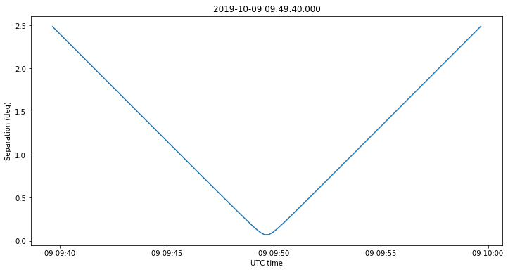
According to the NORAD TLEs, Es’hail 2 was located at an azimuth of 138.92º and elevation of 34.23º as seen from my station. It is assumed that the dish was aimed close to this location, but still we keep in mind a possible pointing error. The figure below shows the separation between the sun and Es’hail 2 on October 9, which was the day of closest separation. The time of closest separation was 09:49:40 UTC. On other days around October 9, the sun also passed nearby Es’hail 2 at around 09:50 UTC, but not so near as on October 9.
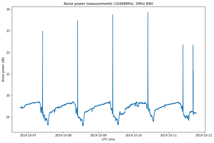
The figure below shows the noise measurements recorded over the course of five days. We see the noise spike up at around 09:50 UTC each day when the sun passes through the beam of the dish. The second spike on October 11 is a Y-factor measurement that will be described later. We observe that the noise changes in a daily pattern due to the LNB gain changing with temperature. We have more noise at night when the LNB is cooler.
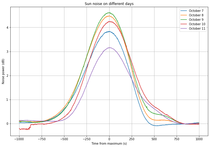
Below we show the observation of the sun noise on each of the five days as the sun passes through the beam of the dish. They observations show sun noise plus “sky” noise (defined as the antenna temperature plus the receiver noise) and they have been scaled to show the sky noise as 0dB. The observations have been arranged so that the maximum is attained at the middle of the graph. The maximum noise obtained is 4.6dB.
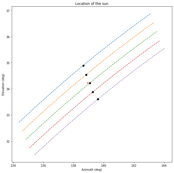
In the figure below we show the location of the sun corresponding to each of the curves in the figure above. The colour coding is the same, so the blue curve corresponds to October 7 and the purple curve corresponds to October 11. The point on each curve where the noise attained its maximum value is shown with a black dot, and the location of Es’hail 2 is shown with a red cross.
Since the days where more noise was measured are October 8 and 9, which showed similar noise values, this means that the location of the dish pointing was approximately halfway between the black dots on the yellow and green curves. This is close to the nominal location of Es’hail 2. The angular separation between the dots on the yellow and green curves is 0.38º. Therefore, an educated guess for the angular distance between the dot on the green curve and the dish pointing is 0.15º.
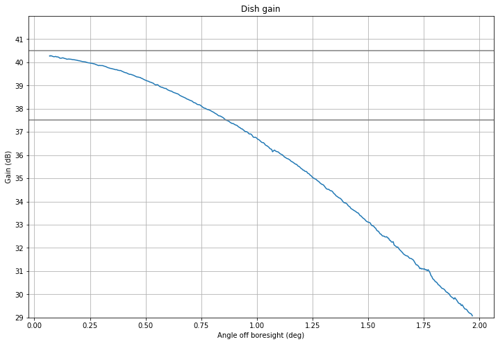
Next, the dish gain is calculated by using the method I described in this post with the sun noise measured on October 9. A gain of 40.5dBi is obtained, with a 3dB half-beamwidth of 0.85º, and a 10dB half-beamwidth of 1.8º. The measured antenna pattern is shown below.
Now we turn to the evaluation of the receiver performance. First we will compute the expected sun noise power at the receiver. The Learmonth observatory gave the following values for the solar radio flux on October 9.
IFLUX : Background Solar Radio Flux
-----------------------------------
Station Date Time Status Freq QS flux Quality
Learmonth 09/10/19 03:24 final 245 13 good
410 26 good
610 34 good
1415 45 ?
2695 66 good
4995 106 good
8800 228 good
15400 554 good

Interpolated value for 1300MHz: 43.7
Interpolated value for 1540MHz: 47.3
Interpolated value for 1707MHz: 50.3
Interpolated value for 2300MHz: 60.1
Interpolated value for 2401MHz: 61.6
Interpolated value for 2790MHz: 67.8
Interpolated value for 5625MHz: 124.5
Interpolated value for 6000MHz: 135.8
Interpolated value for 8000MHz: 200.4
Interpolated value for 8200MHz: 207.2
Interpolated value for 9410MHz: 253.6
Interpolated value for 10400MHz: 297.2
Thus, we take as 297.2Jy the solar flux at the observing frequency of 10488MHz.
The aperture \(A\) of the receiving antenna can be computed in terms of its gain as\[A = \frac{G\lambda^2}{4\pi},\]where \(G\) is the gain and \(\lambda\) is the wavelength. With the gain of 40.5dBi we have measured above, we obtain an aperture of 0.73\(\mathrm{m}^2\).
The efficiency of the dish is defined as the aperture divided by the physical dish collecting area. We can give a rough estimate for the collecting area by assuming that the dish seen from boresight looks as a circle of radius \(r = 0.6\mathrm{m}\), so its area is \(\pi r^2\). Using this estimate for the area we obtain an efficiency of 0.65, which is typical for an offset dish.
The power spectral density of the sun noise received at the LNB probe can be computed as\[P=\frac{1}{2}\gamma FA,\]where \(F\) denotes the radio flux in \(\mathrm{W}/(\mathrm{m}^2·\mathrm{Hz})\), and \(\gamma\) is a dimensionless quantity that accounts for losses, to be described later. The factor 1/2 accounts for the fact that the probe only receives one polarization, while the radio flux is unpolarized.
We now break up the parameter \(\gamma\) into the different losses that are present in the system. First, we have the atmospheric losses \(\gamma_a\). A simple model is given in this article:\[\gamma_a = \gamma_{a,z}^{\frac{1}{\sin \varepsilon}},\]where \(\gamma_{a,z}\) denotes the zenith attenuation, which has a typical value of -0.22dB at 10GHz and \(\varepsilon\) is the elevation. For an elevation of 34.23º we obtain \(\gamma_a = -0.39\mathrm{dB}\).
Next, we have losses \(\gamma_c\) due to the plastic dust cover of the LNB. These are estimated in the article as -0.1dB. Another loss we need to consider is the losses \(\gamma_p\) due to pointing error. For the pointing error of 0.15º we have estimated above, the antenna gain has been reduced by some 0.4dB, so we set \(\gamma_p = -0.4\mathrm{dB}\).
Finally, this other article gives a beamsize correction that should be used when the sun occupies a considerable portion of the antenna beam. The correction can be modeled as the loss factor\[\gamma_b = (1+0.38(w_s/w_a)^2)^{-1},\]where \(w_s\) is the diameter of the radio sun, which is 0.5º for frequencies above 3GHz, and \(w_a\) is the antenna 3dB beamwidth, which is 1.7º in our case. Thus, we obtain \(\gamma_b = -0.14\mathrm{dB}\).
Therefore the total losses are \(\gamma = \gamma_a \gamma_c \gamma_p \gamma_b = -1.03\mathrm{dB}\).
Using the formula above, we obtain a power spectral density of \(8.55\cdot 10^{-21}\mathrm{W}/\mathrm{Hz}\). This can be expressed as a noise temperature in K by dividing by Boltzmann’s constant \(k_B\), obtaining 619K.
Now we compare the sun and “sky” noise (defined as the noise received when the sun is not present in the beam). We interpret these in terms of signal to noise ratios, with the sun noise being the signal and the sky noise being the noise. We have obtained a signal plus noise to noise ratio of 4.6dB. This gives a signal to noise ratio of 2.77dB. Dividing the sun noise by this signal to noise ratio, we obtain a sky noise of 327K.
Let us now study whether this value of 327K for the sky noise is reasonable. On October 11, a Y factor measurement was made where the LNB was pointed to the (hot) ground and the noise power was compared with the (cold) sky noise. A Y factor, or difference, of 2.9dB was measured between the hot and cold temperatures. The ambient temperature was 21ºC, so the hot temperature was \(T_h = 294\mathrm{K}\). The Y factor relates the hot temperature \(T_h\) and the cold temperature \(T_c\), which is mainly due to dish spillover (it also includes the cosmic microwave background) by\[T_h + T_s = Y(T_c + T_s),\]where \(T_s\) denotes the system noise temperature, which is dominated by the LNB noise temperature. The sky noise we have determined above is simply \(T_c + T_s\).
Now, obtaining a good estimate of \(T_c\) is difficult, since the spillover depends greatly on how well the dish is illuminated. In a previous post I had used an estimate of 70K for the spillover, which was taken from the experiments by Ian Roberts ZS6BTE. However, if we accept as valid the sky noise value of \(T_c + T_s = 327\mathrm{K}\) given above, we can solve for the system noise as \(T_s = Y(T_c + T_s) – T_h = 346\mathrm{K}\). This is impossible, since it would imply \(327\mathrm{K} = T_s + T_c > T_s = 346\mathrm{K}\).
This means two things. First, that we have understimated somewhat the losses when computing the power spectral density of the sun noise. As an example, with an additional -0.5dB of losses we would get a sky noise of 292K, which gives a system noise of 276K and a cold temperature of 15K due to spillover. The second thing is that the spillover can’t possibly be as large as 70K. This would mean that we have greatly understimated the losses. Indeed, if instead of an additional -0.5dB of losses we consider -1.5dB of additional losses, we get a sky noise of 232K, a system noise of 159K and a cold noise of 72K. Thus, it seems more likely that the spillover is around 15K (which is what some other authors consider) rather than 70K.
The system noise temperature of 276K obtained above corresponds to a noise figure of 2.9dB, which seems rather high for an LNB, but it is not so surprising, because the experiments by Ian Roberts show that the noise figure of Ku-band LNBs degrades quickly below approximately 10.6GHz, as they are designed to work from 10.7GHz to 12.75GHz.
There are some additional -0.5dB of losses that should be accounted to explain correctly the results of the sun observation. My impression is that perhaps the gain of the dish is not as high as 40.5dB, and maybe is 0.2 or 0.3dB lower than this. Also, the beamsize correction \(\gamma_b\) is computed for a situation with no pointing error. Note that if we point with an error of 0.15º, one side of the limb of the sun is already at 0.35º off boresight, in comparison to 0.25º for a perfect pointing. If we compare the gain pattern at 0.35º and 0.25º, we see that they differ by 0.3 or 0.4dB, so the beamside correction \(\gamma_b\) should be larger if there is pointing error.
Following the first alpha, I have released today v3-alpha1, the second alpha for gr-satellites 3. As I introduced in September, gr-satellites 3 will be a large refactor of gr-satellites, bringing many UI and under-the-hood changes. I am releasing a series of alphas during the development to get feedback from users. Each of the alphas focuses on a different aspect.
The second alpha is focused on input and output formats. New functionality has been implemented to allow the user to choose the input and output in a flexible way. This post describes the main features added.
Running gr_satellites
There is an important change in the usage of the gr_satellites command line tool with respect to alpha0. The syntax for running gr_satellites is now
gr_satellites SATELLITE [additional arguments]
This means that the satellite needs to be specified first, by using either its name, its NORAD ID, or a path to a satellite YAML file, as explained in my post about alpha0.
The reason for this change is that now there are some arguments that depend on the satellite you choose. For example, if the satellite uses FSK, you will get arguments relevant for FSK demodulation, whereas if the satellite uses BPSK, you will get arguments relevant for BPSK demodulation.
In this way, if you just run
gr_satellites -h
you will get a brief summary of options which are applicable to all satellites. However, if you run
gr_satellites GOMX-3 -h
you will get all the options which can be used with GOMX-3.
Input formats
There are two new features regarding input formats in alpha1. The first is IQ input, which is enabled with the --iq argument. Until now, gr-satellites has used real input. This new option allows the use of IQ both with the UDP input and with the WAV file input.
There is an important semantics change when using IQ input with FSK and similar frequency modulation modes. When using real input, gr-satellites assumes that the input is already FM-demodulated (this is indicated in the gr-satellites README by saying “You must use FM mode to receive this satellite”). With IQ input, gr-satellites assumes that the input is not FM-demodulated (as it should be the case with a normal IQ recording), and performs FM demodulation.
For BPSK (which is now implemented in alpha1), there are slightly different semantics between IQ input and real input. For IQ input the signal is assumed to be centred at 0Hz, while for real input the signal is assumed to be centred at 1500Hz for baudrates smaller than 2400baud and at 12000Hz for baudrates larger than 2400baud (these are the well known “narrow SSB” and “wide SSB” modes from gr-satellites 1). This can be changed by using the --f_offset argument.
The second new feature is KISS input. Instead of using an input consisting of RF samples, it is also possible to use a file with frames in KISS format. This is useful to decode and show telemetry already recorded to a KISS file, or maybe to submit telemetry to a server from a KISS file. This option is enabled with the --kiss_in argument.
Output formats
The main focus for this alpha is on flexibility in output formats, which was one of my main goals for the gr-satellites refactor. Let us review the output options that are available in this alpha.
By default, gr_satellites will use as output the thing that makes more sense for the satellite selected. If a telemetry definition written in construct is available, the parsed frames will be printed to the standard output. If there is only partial information about the telemetry transmitted by the satellite (perhaps only the headers but not the payload format is known), this will be used to print the data. If there is no information at all, gr_satellites will resort to printing the packets in hex. The output can be redirected to a file instead by using the --telemetry_output argument.
Additionally, if the satellite transmits other data, such as images, gr_satellites will process this data by default (storing and displaying images, for example).
It is possible to switch to hexdump output instead, using the --hexdump parameters. This will print all the packets in hex to the standard output.
In addition to being printed to the screen, the decoded frames can be stored to a KISS file by using the --kiss_out parameters. The file is overwritten, unless --kiss_append is used.
Another kind of output that happens in background is submission to the telemetry servers. gr_satellites always tries to send telemetry to all the applicable servers. These are SatNOGS DB for all satellites, the FUNcube warehouse, for FUNcube satellites, and the PW-Sat2 server for PW-Sat2.
Information needed to submit to these servers is stored in the gr-satellites config file, which is a new appearance in this alpha. This file is located in ~/.gr_satellites/config.ini and its default contents are
For submitting to SatNOGS DB it is necessary to fill in the [Groundstation] information. The submit_tlm parameter can be set to no if the user doesn’t want to submit telemetry, in which case gr_satellites will never submit to any of the servers. For submitting to the FUNcube warehouse it is necessary to fill in the credentials in the [FUNcube] section, while for submitting to PW-Sat2, it is necessary to enter the path to the credentials JSON file in the [PW-Sat2] section.
GRC blocks
Users in interested in building their own GNU Radio companion flowgraphs will find that most of the functionality added to the gr_satellites command line tool is also available as GRC blocks in the form of “components”.
There is now a new BPSK Demodulator in the demodulator components category. Also, the demodulators can be switched between real (float) and IQ (complex) input.
gr-satellites demodulator components
Regarding data source components, there is now the KISS File Source. This can be very useful, as it will read PDUs from a KISS file.
gr-satellites data source components
The data sinks included in this alpha are shown below.
gr-satellites data sink components
The hexdump sink and KISS file sink are very simple sinks that take PDUs and will print them in hex format or save them to a KISS file respectively. The Telemetry Submit sink uses the gr-satellites config file located in ~/.gr_satellites/config.ini to get the user information and credentials.
The Telemetry Parser uses the concept of “telemetry definition”. This is either a construct object or some more complex class supporting the parse() method. The telemetry definition needs to be exported by the satellites.telemetry package (see here). Currently, there are only three telemetry definitions available: gomx_3, sat_1kuns_pf and ax_25, but more will be added in the future. In the Telemetry Parser block one should enter the name of the telemetry definition. For example, ax_25.
Next alpha
There are only four satellites supported in alpha1: 1KUNS-PF and GOMX-3, which were added in alpha0, and US01 and EntrySat, which have been added in alpha1 to test and demonstrate the FSK and BPSK AX.25 decoders.
The next alpha will focus on adding enough infrastructure to support all the satellites that are available in gr-satellites 2. This will probably cause some changes to the format of the satellite YAML files, which is the main reason why I have only written a few satellite YAML files so far (to avoid having to rewrite many files if I change the format).
Interested users will find that gr-satellites alpha1 has enough tools to decode any AX.25 satellite, and may want to try using the US01 (9k6 FSK) and EntrySat (9k6 BPSK) decoders with other AX.25 satellites, or adding new YAML files to support other baudrates.
A while ago I spoke about feeding an external reference to the LimeSDR USB. Now I wanted to use an external reference with the LimeSDR Mini that I have in my QO-100 groundstation to lock all the system to GPS. Preferably I wanted to use 27MHz as the reference, since this is what I am using in my LNB, so this would save me from having to run 10MHz or another frequency to the groundstation.
I wasn’t so sure how well this would work, since there are a few threads with questions in the MiriadRF forums, but I haven’t seen any explaining things in a clear way. There are different anecdotes of things that worked or didn’t work for several people, but not that many definitive answers. Among all the threads, this one seems mostly helpful.
Somewhat surprisingly, everything has worked well on the first try. I am now using a 27MHz external reference with my LimeSDR Mini. Hopefully this post will be of help to other people.
The relevant part of the LimeSDR Mini v1.2 schematic is shown in the figure below (click on it to view it in full size).
LimeSDR Mini v1.2 clock hardware
As we see, there is a 40MHz VCTCXO that feeds an LMK00105 clock buffer. This fans out the clock to different parts of the LimeSDR Mini, including the LMS7002M RFIC (TxPLL_CLK and RxPLL_CLK), the FPGA (LMK_CLK), and the clock output U.FL connector (REF_CLK_OUT).
It is possible to feed in an external clock instead of using the VCTCXO by removing the 0 Ohm resistor R59 and installing R62, which is not fitted by default. The 0 Ohm resistor R62 goes directly to the clock input U.FL connector.
The figure below shows the LimeSDR Mini board. R59 and R62 are located in the smaller red box. There are only three pads for the two resistors, so they share a common pad and it is only possible to install one of them. To switch R59 to R62, it is enough to rotate the resistor in the red box by 90º (so in the figure the resistor would be rotated from a horizontal position to a vertical position).
LimeSDR Mini v1.2 board
This is the only hardware modification that needs to be done. There is also the question of the electrical specifications of the external reference signal. The LMS7002M datasheet says that the chip accepts a PLL reference between 10MHz and 52MHz.
Additionally, we need to take care about what the LMK00105 accepts. Its datasheet says that for a single-ended clock supplied through the CLKin pin, the peak-to-peak voltage swing should be between 0.3V and 2V. Since the clock input connector of the LimeSDR Mini is terminated to 50 Ohms, the clock input should be between -6 and 10dBm.
In my case, I am using a DF9NP PLL to generate the 27MHz reference. This gives a sine output with an open circuit voltage of 3.1V, which would give around 7.8dBm (or maybe a bit less) to a 50 Ohm load. Between the PLL and the LimeSDR Mini I have several metres of 75 Ohm coax and a 3dB splitter, so the clock input to the the LimeSDR mini is probably around 3dBm, perfectly within margins.
Finally, there is the matter of software. The LimeSuite driver needs to know about the reference frequency that you are feeding to the LimeSDR Mini. This is done by calling the LMS_SetClkFreq() function in the LimeSuite API. Probably it is best to do this right after initializing the chip, before setting up the sample rate or LO frequencies. As an example, you can see here how I am doing it in my limesdr_linrad software (which was described in this post).
These are all the steps needed to use an external reference with the LimeSDR Mini. Apparently it is possible to use any external clock between 10 and 52MHz just by changing a resistor and calling an API function. In particular, it is not necessary to modify the FPGA gateware. I understand that there is a NIOS CPU in the FPGA gateware that runs from the reference clock. This means that this CPU will run slower or faster depending on which reference frequency you use, but I don’t think it is a major concern.
Following a long discussion with Bernd Zoelgert DL2BZ about the frequency stability of the local oscillator of the QO-100 narrowband transponder, I have decided to try to measure the Allan deviation of the transponder. The focus here is on short-term stability, so we are concerned with observation intervals around \(\tau = 1 \mathrm{s}\).
Of course, as with any measurement problem, the performance of the measurement equipment should be better than the “device under test”. In this case, to measure the QO-100 LO it is necessary to compare it against a reference clock which is more stable (ideally an order of magnitude better).
My whole station is locked to a DF9NP GPSDO, which is a 10MHz VCTCXO disciplined by a uBlox LEA-4S GPS receiver. That’s great to measure long-term stability, but for short-term measurements you are essentially relying on the stability of the VCTCXO, which is not so great. Therefore, the whole purpose of this experiment is first to determine whether my station is actually able to measure the QO-100 LO or not. Spoiler: it turns out the answer is “no”, as in most articles whose title is phrased as a question.
The main idea of the experiment is to transmit a CW tone through the NB transponder with my station, receive it on the downlink and perform phase measurements of the received tone. In this measurement there are two clocks involved: the reference GPSDO at my station and the QO-100 LO, and the measurement doesn’t tell us anything about how these two clocks compare (i.e., which one is more stable).
To help us with this situation, we rely also on the BPSK beacon. This is transmitted by AMSAT-DL‘s groundstation in Bochum, Germany. The transmitter is locked to a GPSDO of some sort. I can receive the BPSK beacon with my station and perform phase measurements of the BPSK signal.
Before jumping to the measurement setup, let us consider what we can achieve with these two measurements. We are able to measure at my station \(\varphi_{\mathrm{CW}}\) and \(\varphi_{\mathrm{BPSK}}\), the phases of the CW and BPSK signals. There are three clocks involved in the system: the GPSDO at my station, which I will denote as \(t_{\mathrm{EA}}\), the GPSDO at Bochum, which I will denote as \(t_{\mathrm{B}}\), and the QO-100 local oscillator, which I will denote as \(t_{\mathrm{QO}}\).
There are also three frequencies involved in the measurements: the downlink frequency \(f_D = 10489.8\mathrm{MHz}\), the uplink frequency \(f_U = 2400.3\mathrm{MHz}\), and the QO-100 LO frequency \(f_L = f_D – f_U = 8089.5\mathrm{MHz}\).
Writing the phase measurements in units of cycles and ignoring affine terms (which are ignored by Allan deviation), we have\[\begin{split}\varphi_{\mathrm{CW}} &= f_L (t_{\mathrm{QO}} – t_{\mathrm{EA}}),\\\varphi_{\mathrm{BPSK}} &= f_L t_{\mathrm{QO}} + f_U t_{\mathrm{B}} – f_D t_{\mathrm{EA}},\\\varphi_{\mathrm{CW}} – \varphi_{\mathrm{BPSK}} &= f_U (t_{\mathrm{B}} – t_{\mathrm{EA}}).\end{split}\]
As we see, the differential measurement \(\varphi_{\mathrm{CW}} – \varphi_{\mathrm{BPSK}}\) is useful because it cancels the QO-100 local oscillator. Indeed, it gives a clock comparison between the clocks at Bochum and my station made at 2.4GHz. The measurement of \(\varphi_{\mathrm{CW}}\) gives a clock comparison between QO-100 and my station at 8GHz, while the \(\varphi_{\mathrm{BPSK}}\) measurement is harder to interpret, as it involves all three clocks and frequencies.
For the measurement setup, the hardware at my station consists of a DF9NP 10MHz GPSDO, a DF9NP PLL that multiplies the 10MHz reference to 27MHz, an Avenger Ku-band PLL-based LNB which generates a 9750MHz LO from the 27MHz reference, and a LimeSDR Mini clocked off the 27MHz reference that receives at the 740MHz IF and transmits directly at 2.4GHz.
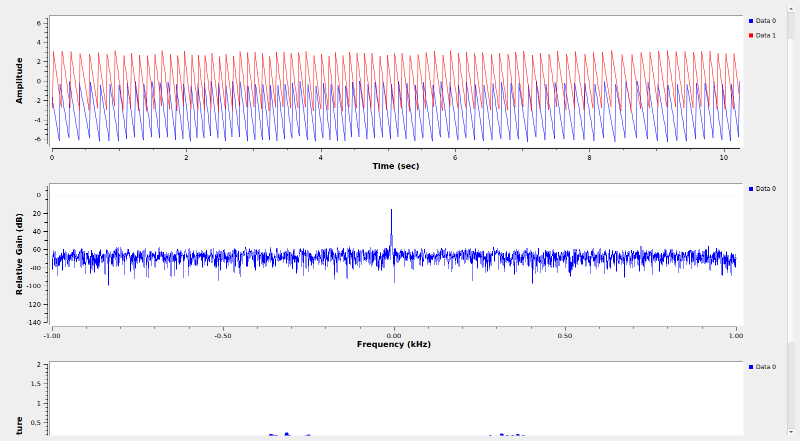
From the software side, I am using my limesdr_linrad tool from the qo100-groundstation repository and GNU Radio. This GNU Radio flowgraph generates the CW tone so that it ends up 5kHz below the BPSK beacon frequency and performs phase measurements of the tone and the BPSK beacon on the downlink. The phase of the tone is measured with a PLL, while the phase of the BPSK beacon is measured with a Costas loop. Phase measurements of each of the signals are written to a file at a rate of 100Hz. The file is then processed in this Jupyter notebook to compute and plot Allan deviation.
The measurement test was made on 2019-11-10, between 11:10 and 11:20 UTC. A continuous CW tone was transmitted approximately 5kHz below the BPSK beacon. Its power was adjusted so that the downlink power was 2dB lower than the BPSK beacon. The phase measurements obtained during the tests are in this file. It is somewhat longer than the 10 minutes that the test lasted “officially”, since I started a bit earlier in order to transmit a CW identification with my callsign and ended up a bit late to transmit another CW identification.
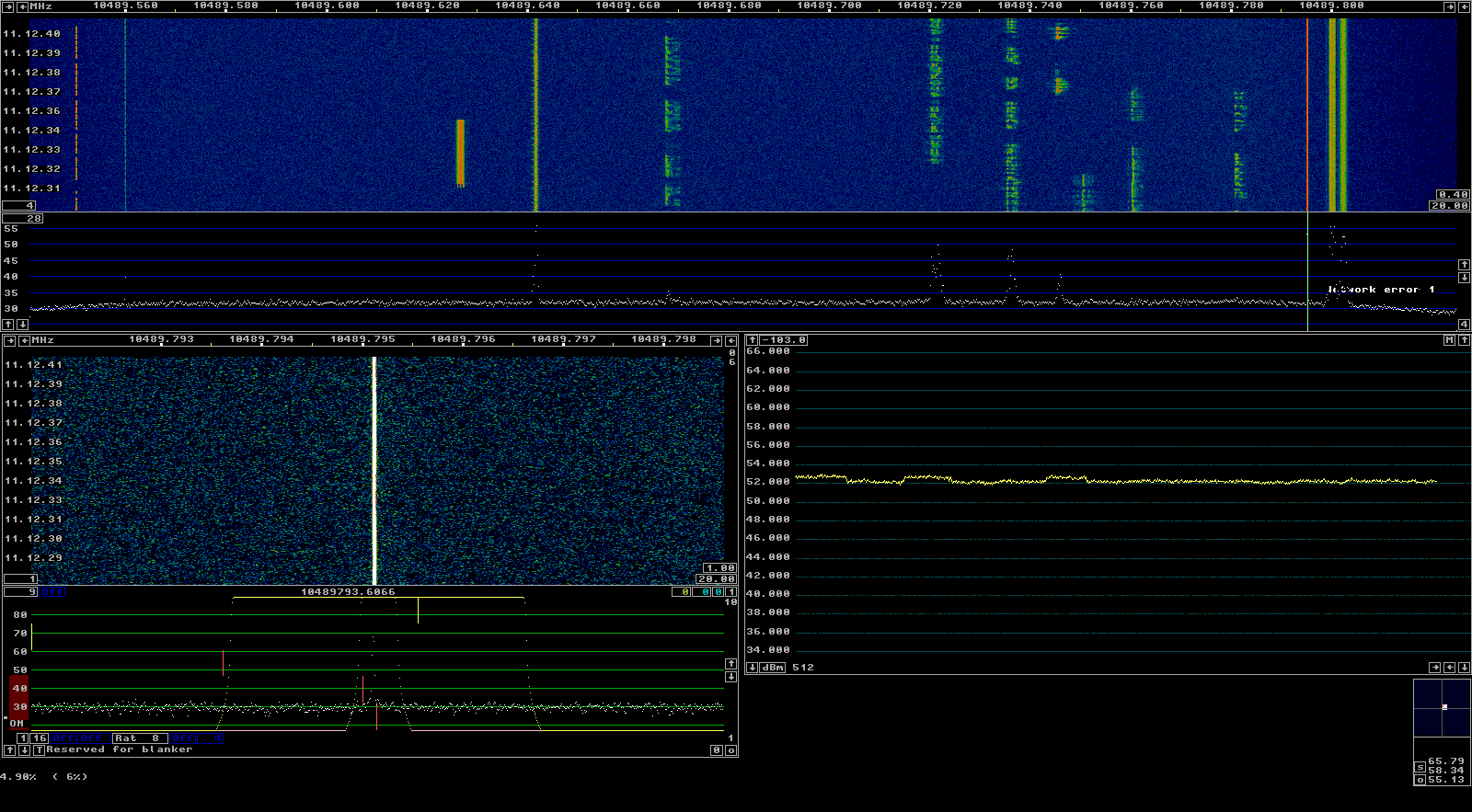
The figures below show the GNU Radio flowgraph performing the phase measurements during the test and Linrad monitoring the transponder downlink. Note that Linrad was only used for monitoring, and not involved in the measurement process.
GNU Radio flowgraph measuring the phase of the BPSK beacon and CW toneTest CW tone being monitored in Linrad
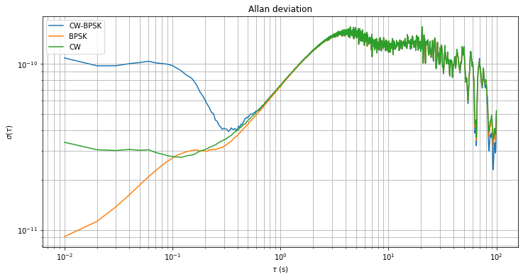
The plot of the Allan deviation of the measurements is shown below. Note that to compute the Allan deviation of a time series of clock comparisons, you need to know the frequency at which these clock comparisons were made. The equations above show that the CW-BPSK measurements were done at a frequency of 2.4GHz, while the CW measurements were done at 8GHz. The BPSK measurements involve several clocks and frequencies, so it is not clear what to do without further considerations. However, if we use 10GHz as the measurement frequency for the BPSK measurements (as done in the plot below), we see that the three traces line up neatly for \(\tau > 0.5\mathrm{s}\).
For the interpretation of these results, first we know that the CW-BPSK and CW measurements have roughly the same deviation. The clock which appears in both measurements is my station’s clock \(t_{\mathrm{EA}}\). This means that my station clock is less stable that the clocks at Bochum or QO-100, so it can’t possibly be used to measure the QO-100 LO. Since \(t_{\mathrm{EA}}\) is less stable than the two other clocks, it is the dominating term in \(\varphi_{\mathrm{BPSK}}\). This justifies our choice of 10GHz as the measurement frequency when computing the Allan deviation for the BPSK measurement, since \(\varphi_{\mathrm{BPSK}}\) turns out to be a measurement at 10GHz of my station’s clock.
In conclusion, my clock is less stable than the clocks at Bochum or QO-100, so the Allan deviation shown for \(\tau > 0.5\mathrm{s}\) is just a measurement of the Allan deviation of my clock. At least this measurements place an upper bound on the stability of the QO-100 local oscillator. We see that it is better (probably much better) than \(7\cdot10^{-11}\) for \(\tau = 1\mathrm{s}\).
There seems to be interesting data about phase noises in the Allan deviation for \(\tau < 0.1\mathrm{s}\), but I haven’t done an interpretation of that data.
It would be interesting if other stations with more stable clocks can participate in this kind of measurements. A good OCXO would be ideal for this kind of short-term stability measurements.
Back in August, I posted about my calculations of the site where DSLWP-B impacted with the lunar surface on July 31. The goal was to pass the results of these calculations to the Lunar Reconnaissance Orbiter Camera team so that they could image the location and try to find the impact crater.
Yesterday, the LROC team published a post saying that they had been able to find the crash site in an image taken by the LRO NAC camera on October 5. The impact crater is only 328 metres away from the location I had estimated.
This is amazing, as in some way it represents the definitive end of the DSLWP-B mission (besides all the science data we still need to process) and it validates the accuracy of the calculations we did to locate the crash site. I feel that I should give due credit to all the people involved in the location of the impact.
Wei Mingchuan BG2BHC from Harbin Institute of Technology was the first to take the orbital information from the Chinese Deep Space Network, perform orbit propagation and compute the crash location assuming a spherical Moon, thus obtaining an approximate position in Van Gent X crater. Cees Bassa from ASTRON refined Wei’s calculations by including a digital elevation model. Phil Stooke from Western University first suggested to use a digital elevation model, helped us contact the LROC team, and filled in an observation request for the camera. And of course the LROC team and the Chinese DSN, since the quality of their ephemeris for DSLWP-B allowed us to make a rather precise estimate.
The LROC team has posted the images shown below, where in a comparison between an image taken in 2014 and the image taken in October the small crater can be seen.
DSLWP-B crash site image
The image of the crash is M1324916226L, an image taken by the left NAC camera. However, I can’t find this image yet in the LROC archive, so it seems this image hasn’t been made public yet.
The small crater, which the LROC team estimate to be 4×5 metres in diameter, is visible more clearly if we compute the difference between the before and after images (an idea of Phil Stooke). The figures below show this difference both as a signed quantity and as an absolute value.
Difference in the before and after imagesAbsolute value of the difference between before and after images
Though my eye fails to see it, the LROC team says that the long axis of the crater is oriented in a southwest-northeast direction. This is consistent with the direction of the impact, since DSLWP-B was travelling towards the northeast.
For the comparison with the October 5 image, the LROC team has chosen an image taken with a similar illumination angle. In fact, the lunar phase in both images only differs in 10º, so the shadows are very similar, with the sun located towards the southwest. In fact, the newest image of the area was taken on 2018-10-16, but the one from 2014 probably gave the most similar illumination conditions.
In my post in August I included a link to Quickmap showing the estimated area of the impact. Now I have marked in red the location of the crash. For a sense of scale, the large crater northwest of the crash is some 50 metres in diameter. You can see both points in Quickmap here.
Location of DSLWP-B crash (red) and estimate (blue)
It is good to go back to all the simulations I did to have an idea of what the 328m error represents. My final simulation was done with the ephemeris from July 25, so they were 6 days old at the moment of impact. When I used the ephemeris from July 18, the position of the impact changed by 231m, while the ephemeris from June 28 yielded a change of 496m. Therefore, it seems that an error of 300m is well in line with what we could expect of the precision of the Chinese DSN ephemeris.
The impact location computed by Cees Bassa was 2786m away from my estimate. The main problem with Cees’s estimate is that the orbital model he used considered spherical gravity for the Moon, while my studies showed that it was important to consider non-spherical gravity.
I did most of my simulations with a 10×10 spherical harmonic model for the Moon gravity, but to assess whether this was enough, I also made a simulation with a 20×20 spherical harmonic model. This yielded an impact point which was 74m away from the impact computed with the 10×10 model.
According to my Monte Carlo simulations with a 1km ephemeris error, the 1-sigma ellipse semi-axes of the impact position were 876m in the northeast direction and 239m in the southeast direction. With this information, I gave an educated guess of the position error of 600m in the northeast direction and 200m in the southeasth direction. The actual impact point is 328m northwest of my estimate, so somewhat higher than my error estimate but still within the 2-sigma ellipse. This leaves me quite happy with the quality of my estimate.
A few days ago I tried to measure the QO-100 NB transponder LO stability using my DF9NP 10MHz GPSDO. It turned out that my GPSDO was less stable than the LO, so my measurements showed nothing about the QO-100 LO. Carlos Cabezas EB4FBZ has been kind enough to lend me a Vectron MD-011 GPSDO, which is much better than my DF9NP GPSDO and should allow me to measure the QO-100 LO.
Before starting the measurements with QO-100, I have taken the time to use the Vectron GPSDO to measure the Allan deviation of my DF9NP GPSDO over several days. This post is an account of the methods and results.
The DF9NP GPSDO is based on a 10MHz VCTCXO phased locked to an 800Hz signal coming from an uBlox LEA-4S GPS receiver. Since it doesn’t use an OCXO, it is inexpensive, doesn’t use much power and locks relatively fast. However, its stability is not as good as that of an OCXO-based GPSDO. In my experiments with QO-100 I measured an Allan deviation of \(10^{-10}\) for \(\tau\) between 1 and 10 seconds, which is typical of a TCXO.
The Vectron GPSDO that I’m using is the C6300 series evaluation kit for the MD-0113-BXJ-DAOC. Its datasheet advertises an Allan deviation of \(10^{-11}\) for \(\tau = 1\mathrm{s}\) and \(2\cdot 10^{-11}\) for \(\tau = 10\mathrm{s}\), and great holdover characteristics. It has been running for a couple of days before the start of the experiment, and so it has surveyed in the position of my GPS antenna and it is using a fixed position for its navigation solution.
Both GPSDOs are connected to the same GPS antenna via an (improperly terminated) T-connector. The antenna is a simple patch antenna and is located in a less than ideal position, near the ledge of a north-facing window, so it has only partial view of the southern sky.
I am using a LimeSDR-USB to compare the phases of the GPSDOs 10MHz outputs. To do so, the DF9NP GPSDO 10MHz output is used as an external reference in the LimeSDR as described in this post. The 10MHz output of the Vectron GPSDO is connected to the RF input of the LimeSDR through sufficient attenuation. This attenuation is provided by a Mini-Circuits ZFDC-10-1 directional coupler as follows: the OUT port is connected to the GPSDO 10MHz output, the IN port is terminated with a 50 Ohm load, and the CPL port is connected to the LimeSDR-USB. This is another less than ideal solution, but it gives lots of attenuation.
The LimeSDR-USB is tuned to 9.9MHz with a sample rate of 2Msps. This is possible by setting the LO to 30MHz, running with 32x oversampling, so the DAC rate is 64Msps, and using the NCO at -20.1MHz. This allows us to receive the 10MHz signal from the Vectron GPSDO at 100kHz in the IQ baseband.
A GNU Radio companion flowgraph is used to lock a PLL to the signal and take phase measurements. A bandwidth of 10Hz is used for the PLL and the phase measurements are taken at a 100Hz rate. These are saved to disk for later analysis. The GRC flowgraph can be downloaded here and is shown in the figure below.
GNU Radio flowgraph for phase comparison of 10MHz GPSDOs
According to the phase measurements, the Vectron GPSDO signal is not exactly at 10MHz. There is an error of approximately 0.168mHz. This is caused by the frequency synthesizers of the LimeSDR: the ADF4002 doesn’t multiply the 10MHz reference coming from the DF9NP GPSDO by 30.72 exactly to yield the 30.72MHz LMS7002M clock, and likewise, the LMS7002M doesn’t multiply its 30.72MHz clock exactly by 30/30.72 to yield the 30MHz LO. Moreover, the NCO doesn’t run exactly at -20.1MHz, and the sample rate is not exactly 2MHz. Therefore, the 10MHz signal from the Vectron ends up with some small frequency error in the IQ baseband. This doesn’t affect the Allan deviation, however, so we will ignore this effect in the rest of this post.
The measurements were done between 2019-11-17 21:55 and 2019-11-20 18:15 UTC. However, there are phase jumps around 2019-11-20 04:58:00 UTC, most likely because the DF9NP GPSDO lost GPS lock at that moment. For simplicity, only the segment of measurements between 2019-11-17 21:55:31 and 2019-11-20 04:57:30 is used in the analysis. This amounts to almost 200000 seconds worth of measurements.
The figure below shows the phase difference between the two 10MHz signals after removing the linear drift caused by the instrumental 0.168mHz offset. The RMS phase difference is 14ns, and occasionally we get differences up to 80ns. This is well in line with the usual performance of the 1PPS (or other timepulse signal) of a non-timing-grade GNSS receiver, so we can expect this kind of performance from the DF9NP GPSDO.
The figure below shows the Allan deviation computed using the method of overlapping segments. In blue we show the measurements obtained in this post, while in orange we show a clock comparison between the DF9NP GPSDO and the GPSDO at the QO-100 groundstation in Bochum (Germany) done over the QO-100 NB transponder as described in this post. Both traces measure the performance of the DF9NP GPSDO, since the Vectron and the Bochum GPSDOs are much better.
The same kind of behaviour appears in both traces, although the orange trace is slightly lower. This might be caused by the different instrumental setup used in each of the measurements. The blue trace was obtained at an observation frequency of 10MHz, while the orange trace was obtained at an observation frequency of 2.4GHz using an S/X satellite link.
The longer measurement span done in this post shows the Allan deviation up to \(\tau = 10^5\mathrm{s}\). We see that for \(\tau > 10^2\mathrm{s}\) the GPS disciplination kicks in and the Allan deviation decreases by an order of magnitude per decade. Between \(\tau = 1\mathrm{s}\) and \(\tau = 10^2\mathrm{s}\) we see an Allan deviation around \(10^{-10}\), dominated by the stability of the TCXO.
The calculations and figures in this post have been done in this Jupyter notebook.
The Vectron MD-011 has an Allan deviation of \(10^{-11}\) at \(\tau = 1\,\mathrm{s}\) and \(2\cdot10^{-11}\) at \(\tau = 10\,\mathrm{s}\) according to the datasheet, so it is an improvement of an order of magnitude compared to my DF9NP TCXO-based GPSDO. I have made more measurements with the Vectron MD-011 as in my previous experiments, measuring the phase of the BPSK beacon transmitted from Bochum and a CW tone transmitted with my station. This post summarizes my results and conclusions.
Long measurement of the BPSK beacon
The first experiment I did was a long measurement of the BPSK beacon phase. Recall from the previous post that this measurement is harder to interpret, since it involves three clocks measured a different frequencies: my station clock, the clock at Bochum, and the transponder local oscillator. Additionally, for long measurements, the satellite movement with respect to the groundstations needs to be taken into account.
The measurement was done on October 21 and 22, spanning a bit over 41 hours. The test_bpsk_beacon.grc GNU Radio flowgraph was used to recover the carrier phase of the beacon with a Costas loop (with 10Hz bandwidth) and write phase measurements at a 100Hz rate. These measurements are analyzed in a Jupyter notebook.
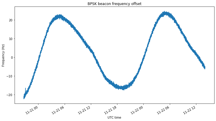
The figure below shows the BPSK beacon frequency offset. The 0Hz level in the graph is set arbitrarily so that the trace is more or less centred at zero. The daily sinusoidal Doppler curve can be seen easily. The frequency averaging period in this graph is 1 second.
The Doppler of Es’hail 2 has been thoroughly studied in several posts in this blog. For instance, this post shows some frequency measurements of the BSPK beacon done back in March. The Doppler curve resembles a sinusoidal curve with a period of one (sidereal) day and an amplitude of approximately 2ppb (or 20Hz). Most of the Doppler on the BPSK beacon is due to the downlink Doppler, owing to the large frequency ratio of 4.37 to one between downlink and uplink frequencies.
The Allan deviation is computed using the method of overlapping segments. It is shown in the figure below.
For \(\tau\) between 1 and 10 seconds the deviation is already limiting the measurement capabilities of the Vectron GPSDO. For \(\tau > 3\cdot 10^2\,\mathrm{s}\) we see the effects of Doppler starting to dominate, increasing the deviation a lot. When \(\tau\) equals one sidereal day, the Allan variance should drop a lot, because of the quasi-periodicity of the Doppler. This effect can be seen at the right-hand side of the figure.
Measurements of a CW tone and BPSK beacon
The next experiments involved the measurement of the phase of the BPSK beacon transmitted by Bochum and a CW tone transmitted by my station simultaneously, in the manner described in this post. Three observations lasting between 14 and 45 minutes were made in different moments of the day on October 22 and 23.
To comply with the requirement to identify the transmissions, my signal consisted of a continuous CW tone transmitted at 2400.295MHz for the phase measurement and a telegraphy signal looping the message EA4GPZ FREQ TEST transmitted 500Hz below the main CW tone. This telegraphy signal was 6dB weaker than the main tone. The downlink power of the main tone was some 3dB weaker than the BPSK signal.
The GNU Radio companion flowgraph test.grc is used to transmit the measurement signal and take phase measurements. The phase of the BPSK beacon is detected with a Costas loop, while the phase of the CW tone is tracked with a PLL. Both use a bandwidth of 10Hz and the measurement frequency is 100Hz. The results are processed in this Jupyter notebook.
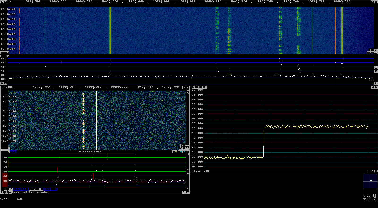
The figure below shows the phase measurement signal during one of the tests.
Phase measurement CW signal shown in Linrad
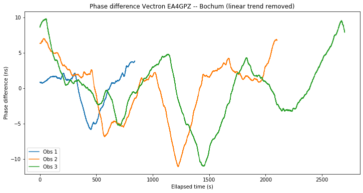
As explained in the previous post, by subtracting the phases of the CW tone and BPSK beacon, a comparison of the clocks at my station and Bochum at an observation frequency of 2.4GHz is obtained. The figure below shows the clock difference in nanoseconds for each of the three observations.
The difference reaches values of up to +/-10ns. This might seem large, since a good GPS receiver can compute a timing solution with a noise of perhaps 2 or 3ns. The reason for the variations much larger than 3ns is interesting. While the GPS solution can be rather precise, it is also very noisy, meaning that it varies significantly from epoch to epoch. If the GPSDO was to follow its timing solution closely, the short-term Allan variance would be horrible. Thus, the GPSDO pulls the OCXO slowly, to keep the short-term Allan variance as good as that of the free-running OCXO.
By letting the GPSDO phase difference grow up to 10ns, the Allan variance is kept smaller than by trying to make the difference as close to zero as possible. The Vectron GPSDO shows this quite well in a screen that shows the output offset with respect the timing solution and the OCXO DAC voltage. The offset often reaches 10ns, and the DAC voltage changes only after several seconds.
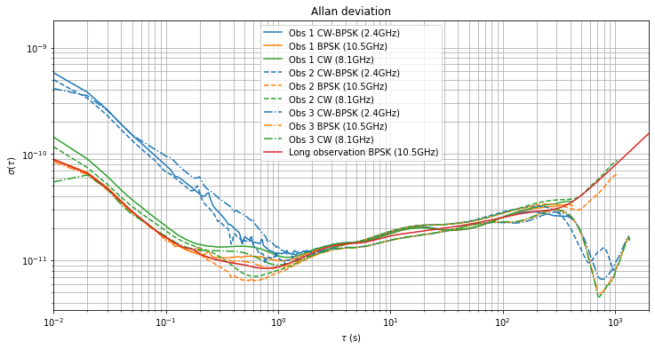
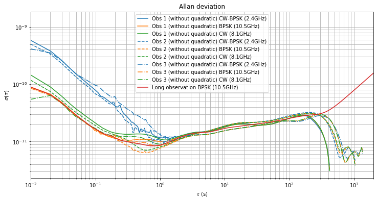
To analyse the Allan deviation we follow the same approach as in the previous post, except for the fact that the method of overlapping segments is used. The difference between the CW tone and the BPSK beacon is considered as a clock comparison between my station and Bochum at a frequency of 2.4GHz. The CW tone is considered as a clock comparison between my station and the QO-100 NB transponder local oscillator at a frequency of 8.1GHz. The BPSK frequency involves the three clocks at different frequencies, and is considered at a frequency of 10.5GHz (as the expression involves my station clock at this frequency).
The Allan deviation of the three observations is shown below. For reference, the deviation of the long observation of the BPSK beacon is shown in red.
Between \(\tau = 1\,\mathrm{s}\) and \(tau = 2\cdot10^2\,\mathrm{s}\) we get roughly the same results in all the observations and for all the three measurements (CW-BPSK, BPSK and CW). According to the discussion in the previous post, this means that the clock at my station is again the least stable clock in the system. This has come to me as a surprise.
After obtaining these results, I have asked Achim Vollhardt DH2VA what kind of GPSDO is used to generate the BPSK beacon in the AMSAT-DL groundstation in Bochum. He tells me that it is an HP Z3801A. This information also appears in the description of the hardware at the Bochum 20m antenna.
Apparently the Z3801A is one of the best GPSDOs ever made, and its Allan deviation at \(\tau = 1\,\mathrm{s}\) can reach \(10^{-12}\). This page shows an Allan deviation plot of the Z3801A, both locked and unlocked, and this page compares the Allan deviation of several unlocked Z3801A units. In view of these results, it is quite likely that the Bochum clock has an Allan deviation around or below \(10^{-12}\), so it is an order of magnitude better than the Vectron GPSDO I’m using.
Often the short-term stability of an OCXO is quoted to be \(10^{-11}\), so in this respect the OCXO in the Vectron GPSDO is average. It seems that the Z3801 uses a really good OCXO that in many units achieves performance around \(10^{-12}\). It is hard to beat this stability for \(\tau = 1\,\mathrm{s}\). A Rubidium standard will be around \(10^{-10}\) for short-term, and a Cesium standard will often be at \(10^{-12}\). A Hydrogen maser is needed to get significantly below \(10^{-12}\).
The details about the clock used in the QO-100 transponder are under NDA. The results of my experiments show that it is probably well below \(10^{-11}\) for \(\tau\) between 1 and 100 seconds.
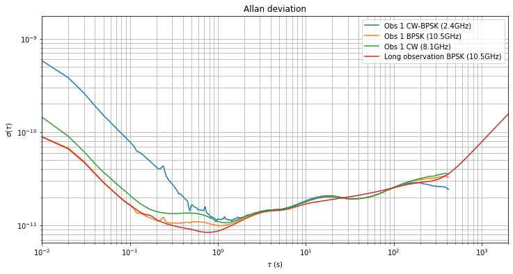
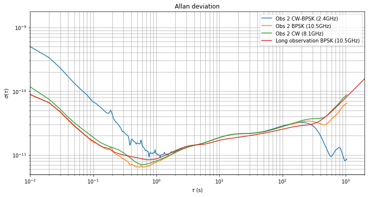
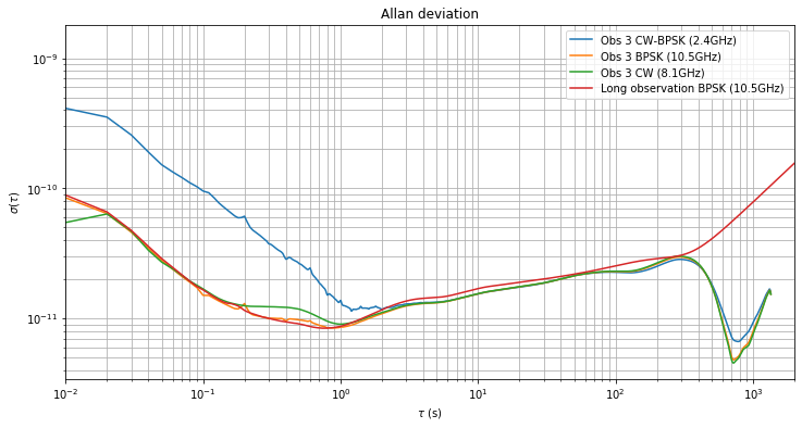
The Allan deviation of each of the observations is shown below in separate figures for an easier comparison. While the first observation is too short to examine the medium-term behaviour for \(\tau\) bewteen \(10^2\) and \(10^3\) seconds, the other two observations show significantly different behaviour. These differences are caused by different Doppler behaviour and will be examined in the next section.
Effects of Doppler on medium-term measurements
We have seen that for \(\tau > 2\cdot10^{2}\,\mathrm{s}\) the effects of Doppler start being noticeable. First let us discuss how each of the three different measurements are affected by Doppler. We denote by \(d_E\) and \(d_B\) the Doppler between Es’hail 2 and my station (EA4GPZ) and between Es’hail 2 and Bochum respectively, measured in parts per one.
For the CW-BPSK measurement, only the Doppler in the uplink legs is important, since the downlink leg is common for the CW and BPSK signals, so the downlink Doppler is cancelled. Also note that the two Dopplers act with opposite sign: a positive \(d_E\) makes the CW signal appear higher in frequency, while a positive \(d_B\) makes the BPSK signal appear higher in frequency. Thus, the total Doppler on the CW-BPSK measurement is \(f_U(d_E – d_B)\), where \(f_U\) is the uplink frequency. Since this measurement is considered at an observation frequency of \(f_U\), the Doppler is simply \(d_E – d_B\).
For the CW measurement, only the Doppler at EA4GPZ plays a role. Since the transponder is non-inverting, the Doppler on the uplink and downlink legs adds up, so the total Doppler is \((f_U + f_D) d_E\). Since this measurement is considered at an observation frequency of \(f_L\), the Doppler is \((f_U+f_D)d_E/f_L\). The factor \((f_U+f_D)/f_L\) is approximately 1.59.
For the BPSK measurement, the Doppler at Bochum plays a role at uplink, while the Doppler at EA4GPZ plays a role at downlink. Both Dopplers act with the same sign: a positive Doppler either at Bochum or EA4GPZ will make the BPSK beacon frequency appear higher. Therefore, the total Doppler is \(f_U d_B + f_D d_E\). Since this measurement is considered at an observation frequency of \(f_D\), the Doppler is \(f_U/f_D d_B + d_E\). The factor \(f_U/f_D\) is approximately 0.229.
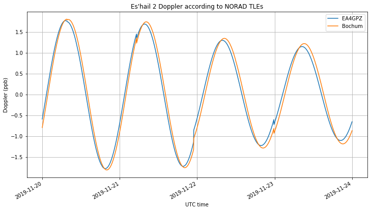
The figure below shows the Doppler at EA4GPZ and Bochum in parts per billion. We see that the Doppler curves are very similar.
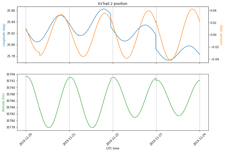
This similarity is caused by the motion of Es’hail 2 and the geometry between the stations and the satellite. The motion of Es’hail 2 is shown below in latitude, longitude and altitude coordinates. We see that its motion is a sinusoidal curve with an amplitude of 0.04 degrees in latitude and longitude, which corresponds to 27km at an orbital radius of 38000km, and 7km in altitude.
However, taking into account the geometry of the problem, we see that most of the Doppler comes from the variations in altitude, and so the Doppler is similar for all stations in the footprint. Since the Earth radius is small compared with the orbital radius, the line-of-sight vector for any groundstation is close to the vector between the Earth centre and the satellite. Indeed, all the groundstations lie within 9.7º off-nadir as seen from the satellite.
This means that the effect of horizontal (latitude and longitude) movement on the Doppler is reduced significantly. Moreover, Madrid and Bochum are relatively close, so the Doppler due to horizontal movement seen in both stations is similar. More information about the effect of Es’hail 2 movement in Doppler can be found in this post.
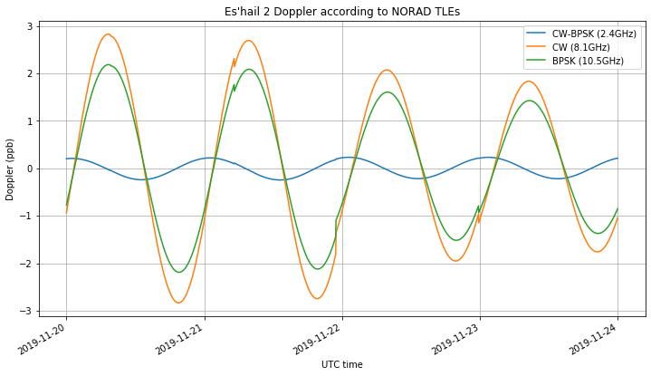
Taking into account the remarks above about how Doppler affects each of the three different measurements, we get the following figure. Since the CW-BPSK Doppler equals \(d_E – d_B\) and \(d_E\) and \(d_B\) are similar, it is much smaller than the others. Assuming that \(d_E = d_B\), we have that the CW Doppler is 1.29 times the BPSK Doppler.
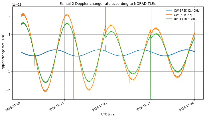
Allan deviation is not sensitive to frequency offset, but rather to frequency drift. Therefore, it is affected by Doppler change rate. In fact, for a frequency drift of \(a\) 1/s, the Allan deviation is \(a\tau/\sqrt{2}\). The figure below shows the Doppler change rate that affects each of the measurements. For the CW and BPSK measurement the change rate peaks at around \(10^{-13}\). Therefore, for \(\tau = 10^{2}\) the effects of Doppler start to be on the order of \(10^{-11}\) and are thus visible in the Allan deviation. The Doppler in the CW-BPSK measurement is much smaller.
The figures shown above have been obtained in this Jupyter notebook.
For medium-term measurements the Doppler change of rate can be assumed to be constant. Therefore, it can be estimated and removed by fitting a degree 2 polynomial to the phase measurements. As shown in the figure below, if we remove this quadratic term from the phase measurements, the Allan deviation of all the observations now decreases for \(\tau\) greater than \(2\cdot 10^2\,\mathrm{s}\), since most of the contribution of Doppler has been cancelled.
Observation 1 is perhaps too short for a good estimation of the frequency drift due to Doppler, but observations 2 and 3 give the following good estimates of the drift in units of 1/s:
We see that there is a difference of an order of magnitude in the drift of the BPSK and CW measurements between observations 2 and 3. The reason is that the observations were done at different moments of the Doppler curve. Observation 2 was made on 2019-11-22 22:08 UTC, when Doppler change rate was high. Observation 3 was made on 2019-11-23 17:10 UTC, when Doppler change of rate was low.
This explains the difference in the Allan deviations of observations 2 and 3. For observation 2, the Doppler in the BPSK and CW measurement is large and appears in the Allan deviation. However, the Doppler in the CW-BPSK measurement is too small to be noticeable, except for \(\tau > 6 \cdot 10^2\), when the deviation starts increasing again. In observation 3, the Doppler in all the three measurements is small, so the deviation decreases until \(\tau = 7\cdot 10^2\), when it starts to increase again.
Concluding remarks
These experiments have shown that the short-term stability of the QO-100 NB transponder local oscillator is better than \(10^{-11}\), so the Vectron MD-011 cannot be used to measure it. The GPSDO at Bochum seems much better than \(10^{-11}\), so perhaps measurements of the transponder local oscillator can be done by receiving the BPSK beacon at Bochum.
The short-term stability of the QO-100 NB transponder local oscillator is better than that of most Amateur stations. The idea to measure the stability of the transponder LO started with some questions from Amateurs interested in running VARA and other OFDM modes which need a lot of frequency stability through the transponder. These measurements show that the transponder is not the limiting factor when using modes that need frequency stability.
The effect of Doppler in the measurements has been studied. The frequency drift \(a\) is on the order of \(10^{-13}\) 1/s and contributes to the Allan deviation as \(a\tau/\sqrt{2}\), so for the measurement precision of \(10^{-11}\) that we are analysing here it starts playing a role for \(\tau > 100\,\mathrm{s}\). For a study down to \(10^{-12}\), the Doppler needs to be taken into account for \(\tau > 10\,\mathrm{s}\). However, for medium-term measurements the Doppler change rate can be assumed constant and cancelled by subtracting a quadratic term from the phase measurements.
The experiments about measuring the frequency stability of the local oscillator of the QO-100 NB transponder with a Vectron MD-011 GPSDO I made a few days ago indicated that the Allan deviation of the local oscillator was probably better than \(10^{-11}\) for \(\tau\) between 1 and 100 seconds. The next step in trying to characterize the stability of the local oscillator is to use a reference clock which is more stable than the Vectron.
I contacted Achim Vollhardt DH2VA asking him if it was possible to record the downlink of the BPSK beacon at Bochum, so as to have a recording referenced to the Z3801A GPSDO in Bochum, which is much more stable than the Vectron. He and Mario Lorenz DL5MLO have been very kind and they have taken the effort to make a recording for me. This post is an analysis of this recording made at Bochum.
The equipment used at Bochum is as follows. A HP Z3801A GPSDO is used as a 10MHz reference. An Octagon LNB is used for downlink reception with a 27MHz reference generated by a DF9NP PLL connected to the GPSDO. The IF from the LNB comes into an AMSAT-DL downconverter, also referenced to the 10MHz GPSDO, and the output of that comes into an Airspy.
The external clock input of the Airspy is connected to the 10MHz GPSDO, but Mario is not sure if this is enabled properly, as he can’t find an option in the software (it might be enabled automatically by the hardware). I couldn’t find anything helpful on the internet either. In any case, after seeing the results of the test, it seems that either the Airspy was indeed locked to the GPSDO or that at the IF it is running its stability doesn’t spoil the Allan deviation.
The recording was made on 2019-11-24 22:45:50 UTC and lasted for 956 seconds. The format was IQ at 39062sps, with the BPSK beacon centred near 0Hz.
The Z3801A GPSDO used at Bochum was provided by James Miller G3RUH. He has sent me the figure shown below, which depicts the Allan deviation of the unit that is running in Bochum. We see that the deviation is around \(3\cdot 10^{-12}\) or \(4\cdot 10^{-12}\) for the range of \(\tau\)’s we are measuring in these experiments.
The recording has been processed with the GNU Radio companion flowgraph test_bochum.grc to obtain phase measurements. As usual, a Costas loop with a bandwidth of 10Hz is used to recover the suppressed carrier, and phase measurements at a rate of 100Hz are stored in a file. This file is then analysed with this Jupyter notebook.
Since in this experiment the transmitter and receiver of the BPSK beacon are both locked to the same clock, the interpretation of the results is simple: as explained in this post, it can be understood as a clock comparison between the Bochum GPSDO and the QO-100 NB transponder local oscillator at a frequency of 8089.5MHz.
The phase difference between the QO-100 local oscillator and the clock at Bochum after removing a linear trend due to frequency offset is shown in the figure below. The quadratic trend is caused by the movement of the satellite. The effects of Doppler in these kind of measurements were treated in my previous post.
Since the observation is short (slightly less than 1000 seconds), we can assume that the frequency drift due to Doppler is constant. Therefore, we can remove the Doppler by fitting a degree two polynomial to the phase difference shown above. The results are shown in the figure below. The frequency drift due to Doppler is \(4.5\cdot 10^{-14}\, 1/\mathrm{s}\). According to the theoretical study I did in the previous post, this is a typical value for the Doppler change rate. An improved measurement could be done at the moments when the Doppler change rate is zero, which happens twice a day.
The phase differece only drifts to +/-0.4ns, which is much better than the results obtained with the Vectron MD-011 GPSDO, so we already see that the Z3801A is much more stable.
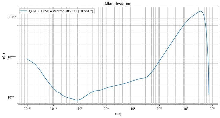
The Allan deviation both for the measurements without removing the quadratic term (blue) and with the quadratic term removed (orange) are shown below. We see that for \(\tau\) between 1 and 10 seconds the Allan deviation is between \(2\cdot 10^{-12}\) and \(3\cdot 10^{-12}\).
For the blue trace, the frequency drift due to Doppler starts playing a significant role for \(\tau > 30\,\mathrm{s}\). Indeed, a constant drift of \(a\) in units of 1/s contributes to the Allan deviation as \(a \tau / \sqrt{2}\). Here we have \(a = 4.5\cdot 10^{-14}\, 1/\mathrm{s}\), and we are concerned with stability on the order of \(10^{-12}\), so the Doppler drift starts playing a role for \(\tau\) on the order of 10 seconds.
In the orange trace we see some indication about what the deviation would look like if Doppler was not present. I wouldn’t trust the values for \(\tau > 200\,\mathrm{s}\), where the deviation falls very steeply, as it is likely they are too unrealistic due to the procedure used to remove the Doppler.
My interpretation of the results of these measurements is that the QO-100 local oscillator is at least as stable as the Z3801A, for \(\tau\) between 1 and 100 seconds, and possibly somewhat more stable. The Allan deviation we have measured matches the characterization of the Z3801A done by James rather well. Note that James’ plot only goes down to 10 seconds, where the deviation is around \(2.5 \cdot 10^{-12}\), and we got a deviation of (2\cdot 10^{-12}\) at 10 seconds.
This means that the QO-100 local oscillator has a very good short-term stability. I think it would be hard to find an Amateur station having better stability, and in fact in my quest to measure the QO-100 LO Allan deviation I haven’t found any one yet. Achim points out that a good clock to measure the QO-100 LO would be the Oscilloquartz BV8607, which is below \(10^{-13}\). However these are rather hard and/or expensive to come by.
Many thanks to Achim, Mario, the rest of the AMSAT-DL team, and to James for their collaboration in this series of experiments.
A few days ago, Bert Hubert, the creator of galmon.eu, discovered a sinusoidal oscillation in the clock drift \(a_{f1}\) parameter of the broadcast ephemerides of Galileo satellites. This variation has a frequency that matches the orbital period of 14 hours and 7 minutes. At first, I suggested that it might be caused by relativistic effects, which are given by\[-\frac{\sqrt{\mu}}{c^2}e\sqrt{A}\sin E,\]where \(\mu\) is the Earth’s gravitational parameter, \(c\) is the speed of light, \(e\) is the eccentricity, \(A\) is the semi-major axis, and \(E\) is the eccentric anomaly. In fact, the order of magnitude of the oscillations that Bert was seeing seemed to agree with this formula.
However, then I realised that this relativistic effect is not included in the broadcast clock model. It needs to be included back by the receivers. Therefore, it shouldn’t appear at all in the broadcast clock. Something didn’t seem quite right. This post is an in-depth look at this problem.
First we start by reviewing the relevant theory about relativistic effects in GNSS satellite clocks. The article “Relativity in the Global Positioning System” gives a good overview of relativistic effects affecting GNSS systems. In equation (39) it proves the formula given above for the relativistic effect on the satellite clock due to a non-circular orbit.
When GNSS clocks are modelled, it is common to correct for this effect in the clock observations, so as to remove the effect from the clock model. Doing so has the advantage that this relatively large periodic term is eliminated from the clock model, simplifying clock modelling and analysis. However, the GNSS receiver needs to put back the correction in order to compute the satellite clock correctly.
Regarding the major constellations, GPS, Galileo and BeiDou remove relativistic effects from their broadcast clock models. This is described in Section 20.3.3.3.3.1 of IS-GPS-200K, in Section 5.1.4 of the Galileo OS SIS ICD v1.3, in Section 5.2.4.9 of the BeiDou B1I SIS ICD v.3.0 and in other related BeiDou documents, and in equation (E.4.16) in the RTKLIB manual. In contrast, GLONASS doesn’t remove the relativistic effects from its broadcast clock model.
When performing orbit and clock determination for the production of precise orbit and clock products, such as those listed in the IGS MGEX, the common practice is to remove the relativistic effect from the clock model. Therefore, the relativistic correction needs to be added again when using an SP3 file. More information can be found in equation (E.4.37) in the RTKLIB manual.
Therefore, when studying broadcast clocks or SP3 precise clocks, we expect not to find this relativistic effect, except when dealing with GLONASS broadcast clocks.
In the experiment presented in this post we look at oscillations in the broadcast and SP3 clocks of satellites of all the major constellations with the goal of studying oscillations at a frequency of 1/revolution. The set of data under study is the MGEX BRDC files for the complete month of November 2019, and the final SP3 clocks from CODE ranging between 2019-11-01 and 2019-11-23 (since final products for the last week in November are not available yet).
In order to simplify the experiment, we study a single satellite per constellation. To magnify the effects due to a non-circular orbit, we choose the satellite having the largest eccentricity. For GPS, that satellite is G21, but because of some anomalies explained below, we chose instead G02, the satellite having the second largest eccentricity. For Galileo, we ignore the highly eccentric satellites E14 and E18, due to the difficulties of modelling their orbit accurately. We choose E31, which has the highest eccentricity among the operational satellites. For BeiDou, the satellites having the largest eccentricity are in an IGSO orbit. Due to the radical differences between an IGSO and a MEO orbit, we choose an IGSO and a MEO BeiDou satellite. The IGSO having the largest eccentricity is C06, while the MEO having the largest eccentricity is C11. For GLONASS we choose R16, which has the largest eccentricity.
The amplitude of the relativistic effect in the satellite clock bias for these satellites is as follows:
E31, 0.958 ns
G02, 44.4 ns
C06 (IGSO), 24.1 ns
C11 (MEO), 5.30 ns
R16, 6.10 ns
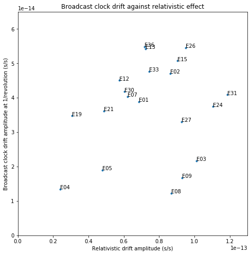
The effect in the satellite clock drift is:
E31, 0.119 ps/s
G02, 6.47 ps/s
C06 (IGSO), 1.76 ps/s
C11 (MEO), 0.717 ps/s
Since the GLONASS broadcast ephemerides don’t include the clock drift parameter, the clock drift of R16 will not be studied.
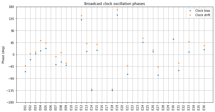
First we look at the clock drift \(a_{f1}\) parameter in the broadcast ephemeris during November. The figure below shows the clock drift for E31 and G02. The average of each trace has been removed to aid visualization.
We clearly see the oscillatory behaviour that Bert first noticed in the Galileo broadcast ephemeris. In contrast, the broadcast clock model for GPS is very simple. The \(a_{f1}\) term is constant except for some jumps every several days.
Next we show the clock drift for the BeiDou satellites. The IGSO C06 has a strong linear trend that has been removed in the plot. We see some large spikes in some of the ephemerides, but no oscillatory behaviour is visible.
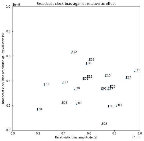
Now we examine the clock bias \(a_{f0}\) parameter in the broadcast ephemerides. We fit and remove a degree 4 polynomial to the data when plotting in order to eliminate long term drift. The figure below shows the clock bias for E31 and G02.
The clock bias of E31 shows the same oscillatory behaviour as the clock drift (but there are other effects, making the graph more noisy). G02 doesn’t show this oscillatory behaviour but shows some noticeable jumps every other day.
The figure below shows the clock bias of the BeiDou satellites. The IGSO C06 has a really large and complex long term drift pattern that is difficult to cancel by fitting a low degree polynomial. The interpretation of this plot is therefore not easy.
Finally, we show the clock bias of the GLONASS satellite R16. Besides a slow variation, the relativistic effect (which is included in the broadcast clock model) can be clearly seen in the graph.
Now we perform a spectral study of the \(a_{f1}\) and \(a_{f0}\) parameters in order to see more easily the oscillations occurring at different frequencies. The figure below shows the spectrum of the clock drift for E31 and G02. The horizontal axis has been normalized to units of 1/revolution (which are different for each constellation, due to different orbital radii).
The oscillatory behaviour that we saw in the time domain for E31 is now clearly seen at a frequency of 1/revolution, with an amplitude of approximately 0.05 ps/s. Note that this is roughly half of the relativistic effect computed above, but I don’t know if this is just a coincidence or if it is significant. A harmonic at a frequency of 2/revolution can also be seen. In contrast, the spectrum of the G02 clock drift doesn’t show any features at integer multiples of 1/revolution.
At this moment it is convenient to remark the effects of unmodelled orbital behaviour in the satellite clock determination. Since unmodelled orbital effects will contaminate the clock determination and these unmodelled orbital effects often happen at frequencies which are integer multiples of 1/revolution, spectral features of the clock model can point to defects in orbit modelling.
Next we study the clock drift of the BeiDou satellites. We see that the MEO C11 doesn’t display any interesting spectral features, while the IGSO C06 has some features at integer multiples of 1/revolution. Probably these are caused by unmodelled orbital effects as remarked above. In contrast to the case of E31, the harmonic at 2/revolution is stronger than the fundamental at 1/revolution.
Below we show the spectrum of the clock bias \(a_{f0}\) parameter of E31, G02 and C11. The spectrum of the IGSO C06 is not shown because it is completely swamped by the slow drift. Here it is clearly visible that E31 is the only satellite which presents oscillations at a frequency of 1/revolution. The amplitude of these oscillations is approximately 0.5 ns, which is roughly half the relativistic effect computed above. Again, I don’t know if this is a coincidence.
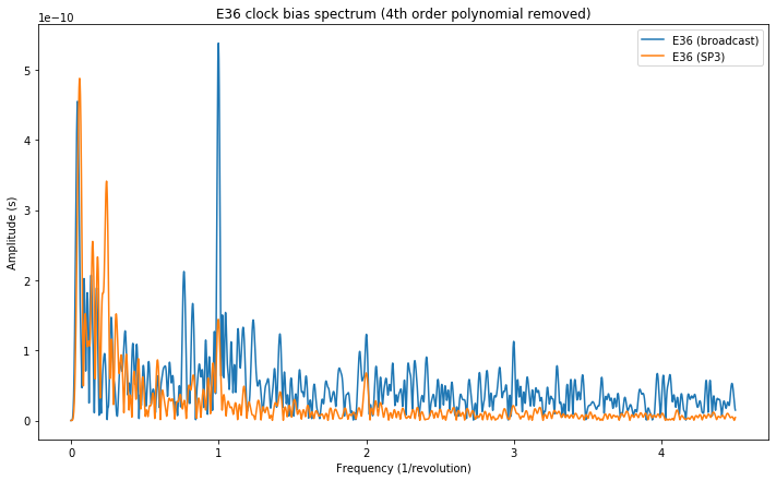
Now we compare the broadcast clocks with the SP3 precise clocks for each of the satellites. The figure below shows the comparison for E31. While the broadcast clock has a strong component at 1/revolution, the SP3 clock has only a weak component at this frequency that can be explained by clock contamination from unmodelled orbital effects. This seems to indicate that the broadcast clock for E31 is wrong: the oscillatory effect that is clearly visible in the broadcast clock is not a real effect of the satellite clock, but rather a problem when computing the broadcast orbit and clocks.
Additionally, we remark that the SP3 clock looks less noisy. This is often the case for precise clocks in comparison to broadcast clocks (and also the 5 minute sampling interval of the SP3 files as opposed to the longer sampling interval of broadcast ephemerides helps average noise out). Because of this, a weak component at 2/revolution is visible in the SP3 clock. Again, this is probably clock contamination.
The figure below shows the comparison for G02. We don’t see any major spectral features. Something small (probably clock contamination) is visible at 2/revolution.
The next figure corresponds to G21 and shows why we have avoided considering this satellite. There are large frequency components in the SP3 file at 1/revolution and 2/revolution that are not present in the broadcast clock. Probably these indicate a problem with the orbit and clock solution that generated the CODE SP3 file. I have decided to discard this satellite rather than investigating this problem further and checking if this effect is also present in the clock solutions computed by other centres.
The clock for the BeiDou MEO C11 doesn’t show any major spectral features, as it can be seen in the figure below.
Finally, we show the clock bias spectrum for the GLONASS satellite R16. The large component at 1/frequency that appears in the broadcast clock doesn’t appear in the SP3 clock. This component corresponds to the relativistic effect, which is included in the broadcast clock but not in the SP3 clock. Its amplitude approximately matches the value of 6.1 ns that we had calculated above.
In summary, this post shows that there is something wrong with the Galileo broadcast clock modelling. The coefficients \(a_{f0}\) and \(a_{f1}\) show some oscillatory behaviour at a frequency of 1/revolution which doesn’t appear in the SP3 precise clocks. While this post only studied the satellite E31, Bert Hubert has observed this effect in other satellites as well. The amplitude of these oscillations is in the same order of magnitude as the relativistic correction of the satellite clock due to a non-circular orbit, but it isn’t equal. The comparison with GPS and BeiDou indicates that this is a problem specific to Galileo.
So far I don’t know anything about the cause of this problem. It might be caused by an incorrect relativistic correction of the observations when performing the orbit and clock determination, to clock contamination due to unmodelled orbital effects (but interestingly nothing seems to show up at harmonics of 1/revolution), or to anything else.
In order to try to shed more light onto the possible cause of the oscillations observed in the previous post, I have now processed the broadcast ephemerides of November for all the active Galileo satellites (including the eccentric E14 and E18) except for E11 and E25, which were out of service at least for some days in November.
This post studies the amplitude and phase of the oscillations of the broadcast clocks at a frequency of 1/revolution. More formally, if we denote by \(x(t)\) the time series corresponding to either the broadcast clock bias or the broadcast clock drift, we compute the complex quantity\[\alpha = \frac{2}{T}\int_{t_0}^{t_0 + T} x(t) e^{-i[n_0(t-t_0) + M_0]}\,dt,\]where \(n_0\) denotes the mean motion in radians/second and \(M_0\) denotes the mean anomaly at \(t_0\) in radians. Note that if\[x(t) = a \cos(n_0 (t-t_0) + M_0 + \varphi),\]then \(\alpha \approx ae^{i\varphi}\), which motivates the definition of \(\alpha\).
When computing \(\alpha\) from the broadcast ephemerides, the mean motion \(n_0\) is taken as the average mean motion among all the ephemerides, while the mean anomaly \(M_0\) is taken as the mean anomaly at the first ephemeris. Note that in all the motivation for this definition we are tacitly assuming that\[n_0(t-t_0) + M_0 \approx M(t) \approx E(t),\]where \(M(t)\) and \(E(t)\) denote the mean anomaly and the eccentric anomaly at time \(t\). This approximation is valid for all the satellites in quasi-circular orbits, but it is not true for the eccentric satellites E14 and E18, for which \(M(t)\) and \(E(t)\) can differ significantly.
In any case, the difference between trying to study \(x(t)\) as a function of \(e^{in_0t}\), as a function of \(e^{iM}\) or as a function of \(e^{iE}\) is not so large. Since \(E\) can be considered as a perturbation of \(M\) and vice versa, the difference is just some kind of phase modulation effect in which energy is lost from the fundamental to form sidelobes, so it will be ignored for the rest of this post.
The complex amplitudes \(\alpha_{\mathrm{bias}}\) and \(\alpha_{\mathrm{drift}}\) are computed as defined above for each Galileo satellite using the broadcast ephemerides transmitted during November. To eliminate long-term effects, a polynomial of degree 4 is fitted and removed from the clock bias time series, and the average of the clock drift time series is also removed. The figure below compares the amplitude \(|\alpha_{\mathrm{bias}}|\) with the amplitude of the relativistic clock bias term for each of the satellites.
Next we compare the \(|\alpha_{\mathrm{drift}}|\) with the amplitude of the relativistic clock drift term.
Additionally, E14 and E18, which do not appear in these graphs, have a very large relativistic amplitude, while the amplitude of their broadcast clock oscillations is similar to that of the other satellites. This was first observed by Bert Hubert.
Therefore, there is no apparent correlation between the relativistic term and the amplitudes of the oscillations of the broadcast clocks. It seems that these oscillations are not related to relativistic effects, or to any other factor depending exclusively on the eccentricity of the orbit.
Since the derivative of \(e^{in_0t}\) is \(in_0e^{in_0t}\) and the clock drift term is supposed to be the derivative of the clock bias term, we expect that \(in_0\alpha_{\mathrm{bias}}\) and \(\alpha_{\mathrm{drift}}\) are similar. The figure below compares \(n_0|\alpha_{\mathrm{bias}}|\) and \(|\alpha_{\mathrm{drift}}|\).
A linear regression is also shown. The slope is 0.6, and the correlation coefficient is 0.85. This is somewhat strange, as we would have expected a slope of one.
Next we compare the phases (complex arguments) of \(\alpha_{\mathrm{bias}}\) and \(\alpha_{\mathrm{drift}}\). In order to obtain a clearer graph, we plot the arguments of \(-\alpha_{\mathrm{bias}}\) and \(-\alpha_{\mathrm{drift}}\) instead (which just corresponds to adding 180º to the argument).
Two things are noteworthy in this figure. First, the difference between the phases of the clock bias and the clock drift is small. Since the clock drift is supposed to be the derivative of the clock bias, we would have expected a phase difference of 90º, so this is rather striking.
Additionally, the phase of most of the satellites is around 0º. Since the orbital radius is proportional to \(1-\varepsilon \cos E\), where \(\varepsilon\) denotes the eccentricity, and we are plotting the phase of \(-\alpha\), a phase close to 0º means that there is a positive correlation between orbital radius and clock bias and drift. As the radius grows, the clock bias and drift both grow.
The figure below shows a linear regression for the phase of the broadcast clock drift in terms of the phase of the broadcast clock bias. The slope is close to one, and the phase difference is approximately -20.4º, with a standard deviation of 11.5º.
While most of the phases of the broadcast clocks are around zero, there are some outliers. The phases of eccentric E14 and E18 are close to -135º. The other outliers are E12 and E19, with phases between 135º and 180º. These satellites are the IOV satellites (recall that the E11, the other active IOV satellite) was not studied since it was unavailable during most of November.
The FOC satellites in quasi-circular orbits have phases around 0º. There is a certain correlation between the phase and in what launch each satellite was put in orbit. The figure below shows the satellites coloured by launch. We see that launches 2015-045, 2017-079 and 2018-060 cluster rather tightly. However, launches 2015-079, 2016-030 and 2016-069 do not cluster so well.
Finally, I have also plotted the spectra of the broadcast and SP3 clock biases and broadcast clock drifts of all the Galileo satellites. The list of all the plots can be found at the end of this Jupyter notebook. We see that the frequency component at 1/revolution is clearly visible in most of the plots of the broadcast clock bias and broadcast clock drift.
Some of the satellites, such as E36 shown below display a noticeable frequency component at 1/revolution in the SP3 clock. This is most likely due to clock contamination from inadequate orbit modelling. However, the component in the broadcast clock is always much larger.
So far it seems that any possible relativistic causes for these broadcast clock oscillations have been ruled out. The most likely case for these oscillations now seems unmodelled effects in the orbit solution contaminating the clock solution, as some people have already suggested.
If this is the case, then these results would indicate that the modelling done by the orbit determination centres that produce the SP3 orbits and clocks is better than the modelling done by the centre computing the broadcast orbits and clocks. Of course this is not a very fair comparison, since the SP3 final solutions are provided after one week, while the broadcast ephemerides are computed in advance.
Additionally, for the sake of fair comparisons it is convenient to mention that it is somewhat more difficult to model the orbits of Galileo satellites in comparison to other GNSS satellites, such as GPS satellites, since the Galileo satellites have a higher cross-section to mass ratio that causes larger solar radiation effects. Also, the cross-section of a Galileo satellite varies noticeably with the orientation, because the body of the satellite is elongated. This means that other GNSS constellations might not display these oscillations in their broadcast clocks simply because their orbit modelling is easier, and not because the models or algorithms used for Galileo are any worse.
In any case, these considerations are at best ramblings without more data supporting the hypothesis that the cause of the oscillations is inadequate orbit modelling. Some of the additional questions that this post raises are why the clock bias and clock drift oscillations do not have the amplitude and phase relationship that one would expect in a derivative, and why there seems to be some kind or correlation between the satellite type (recall that the IOV and FOC satellites are physically very different) and launch, and the phase of the oscillations.
They transmit in the 70cm Amateur satellite band, and although they have beeen successfully coordinated with IARU (see here and here), documentation about the protocols they use has not been published. There is some groundstation software available here, but the interesting part is implemented in the atlgnd_x86_64 and smogpgnd_x86_64 binary executables, for which source code is not available. As far as I know both satellites transmit using the same (or very similar) protocols.
In this post I describe my first attempts at reverse-engineering the transmissions of SMOG-P, with successful results. Preliminary support for decoding SMOG-P and ATL-1 has been added to gr-satellites in the maint-3.8 branch.
The first remark is that even though the IARU coordination sheets state that these satellites use 12.5kbaud GMSK, they are using 1250baud GMSK instead. In fact, for the first day after launch they were using some faster modulation for most of the packets, but they have been changed to 1250baud since Saturday. This change can be observed from the difference in the waterfalls of recordings done before and after the change.
In my first look at the packets, I identified that the 16 bit syncword 0x2DD4 was being used. This is the default syncword for the Si446x family of FSK transceiver chips from SiLabs and is also used in Lucky-7, so most likely the satellites are using this kind of chips. However, a look at the data revealed that it was most likely scrambled.
While trying to get in contact with the satellite team to get some technical details about the scrambler, I decided to take a look at the smogpgnd_x86_64 binary to see if I could pull out any useful details easily.
Here you can see the symbol table of the ELF binary smogpgnd_x86_64 as printed by objdump. There we see numerous references to AO-40, with several functions starting by ao40_ and presumably implementing the different functions of the AO-40 FEC protocol. There are also versions of these functions starting by ao40short_ (more on this later).
Interestingly, there are also functions that apparently perform AES128 encryption and decryption. I find this somewhat concerning. Encryption of Amateur transmissions is forbidden by the ITU Radio Regulations except for the control signals of Amateur satellites. Therefore, it is possible to encrypt telecommands (and perhaps also replies to telecommands from the satellite), but telemetry and other data downlinked from the satellite needs to be sent unencrypted. So far I don’t know if any of the data transmitted by the satellite is encrypted.
I’m also concerned about the origin the code used in smogpgnd_x86_64, since most of the code available online to implement the AO-40 FEC uses a strong copyleft licence. More specifically, the symbol ao40_spiral-vit_scalar.c suggests that code generated by SPIRAL is used in the Viterbi decoder. The code generated by SPIRAL is available under the GPL. The code of Phil Karn’s KA9Q libfec is available under the LGPL. This is also probably reused in smogpgnd_x86_64 (see the symbols ao40_Partab, ao40_decode_rs_8). Therefore, I wouldn’t be surprised if the satellite team is violating some open-source licences by distributing smogpgnd_x86_64 as a binary only.
The symbol table of smogpgnd_x86_64 has been very helpful. It turns out that SMOG-P implements the AO-40 FEC protocol completely, including the distributed syncword. A 5200 bit AO-40 FEC frame is sent as the payload of the packets transmitted by the Si446x. The 0x2DD4 is transmitted automatically by the chip before the payload, but the design intention is probably that the receiver should ignore that syncword and synchronize using the AO-40 distributed syncword.
However, this is not the end of the story. It turns out that SMOG-P transmits frames of three different sizes. These can be seen in the figure below. The frames are the parts of the signal where the amplitude is small. The rest if just noise between frames.
Frames transmitted from SMOG-P, seen in Audacity
The long frames correspond to the 5200 bit AO-FEC frames. There are also some short frames which are approximately half the length of the long frames. This explains the ao40short_ functions, which hint at some modification of the AO-40 FEC protocol for frames of half the size. Perhaps this is achieved by using a single Reed-Solomon (160,128) codeword instead of two, but I will have to take a look at this in more detail.
There are also some very short frames. One of these frames is transmitted at the beginning and at the end of each burst of long or short frames. So far I don’t know anything about them. It is possible that they don’t use any FEC and are intended as some kind of signalling.
A recording of some long frames and of some short and very short frames have been added to satellite-recordings. A decoder for the long frames is now available in gr-satellites. The plan is to add support for short and very short frames once I figure out the details.
I have put a decode of the long frames recorded during the 2019-12-07 19:43 UTC pass on the Budapest University’s groundstation WebSDR in this gist. In a certain sense, the data seems somewhat strange.
In my previous post I talked about the FEC used by the SMOG-P and ATL-1. In there, I reverse-engineered the long frames transmitted by SMOG-P and found that they use the AO-40 FEC protocol.
After publishing that post I started reverse-engineering the short frames. Meanwhile, Peter Horvathpointed me to a Github repository containing an implementation of the FEC used for short frames and long frames. I hadn’t seen that repository before (it’s not easy to search for SMOG-P or ATL-1 in Google, as many unrelated results come up). Indeed this repository contains the source of a FEC decoder for the short frames, so there is no need to reverse-engineer it.
Timur Kristóf, the author of that repository, says that the team plans to release the source for the decoder, but that they are currently very busy with the early operations of the satellites. This is very good news.
I have studied the code in the Github repository and included a decoder for the short FEC frames in gr-satellites.
The short FEC frames are a straightforward modification of the AO-40 FEC protocol. As I suspected, they carry a single Reed-Solomon (160, 128) codeword. The way this is done is by using a 52×51 matrix interleaver instead of 65×80. The length of the distributed syncword is thus 52 bits instead of 65.
However, there is something a little bit strange. Whereas in the standard AO-40 FEC the output of the matrix deinterleaver is sent to the Viterbi decoder after removing the 65 bit syncword, in these short frames the first 80 bits (including the 52 syncword bits) are dropped before sending the frame to the Viterbi decoder. This gives a frame of 2572 symbols to be sent into the Viterbi decoder, which outputs 1283 bits. The last 3 of these bits are dropped to obtain a 160 byte Reed-Solomon codeword.
The list of short frames decoded from the recording I made yesterday can be seen in this gist.
Besides FEC decoding of the short frames, there is still more work to do in order to have a complete decoder. By now I know nothing about the “very short frames” (Timur says that they are used from synchronization). Additionally the format of the data packets is not known. Hopefully this will be made clear when the team releases the source code.
Regarding the AES128 encryption functions that I mentioned in my previous post, Peter stated that the encryption is only used for authentication. I have analyzed the smogpgnd_x86_64 more carefully and I am confident that this is true. The AES128_block_decrypt function is only called from the AES128_builtin_test function, which in turn is not called from anywhere. Additionally, the packets I have decoded don’t seem to be encrypted (the data would appear much more random). Therefore, the downlink doesn’t seem to use any encryption.
The function AES128_block_encrypt function is called from uplink_encoder (which, again, isn’t called from anywhere), so it seems that the uplink uses some form of encryption (perhaps only for authentication). This is perfectly reasonable and follows the ITU regulations, since the uplink is a control signal.
Interestingly, there is also the chk_downlink_pckt_signature. It isn’t called anywhere and just returns -1, so it is not implemented in the binaries released by the team. However this hints that the packets sent by the satellite have some form of authentication. Indeed, in the packets I’ve decoded the last 10 bytes seem quite random. These bytes (or just part of them) might be an HMAC or similar kind of signature.
This form of authentication without data encryption is also allowed by the ITU Radio Regulations, for all forms of communications. It is an interesting concept and it is seldom used in Amateur communications. The most similar thing that I have seen in Amateur radio is the elliptic curve signature in DML. AAUSAT-4 software was also prepared to use a HMAC, but I’ve never checked if the downlink transmissions were signed with the HMAC or it was only for the uplink. Congratulations to the satellite team for bringing in these interesting security features while following the ITU regulations.
The SMOG-P 1P PocketQube that was launched recently has an interesting payload: a UHF spectrum monitor that records power spectral density measurements. Lately, I have been adding support in gr-satellites to decode the telemetry frames transmitted by SMOG-P and ATL-1 (which also carries a similar spectrum monitor), using the code published here as a reference.
As a result of this work, now it is possible to save and plot the spectrum data transmitted by SMOG-P and ATL-1 using gr-satellites. This post explains how.
If you have a look at the smog_p.grc and atl_1.grc flowgraph in gr-satellites, you’ll see a SMOG-P/ATL-1 spectrum save block, shown below.
SMOG-P/ATL-1 spectrum save block
This block saves the spectrum data received in the telemetry into different files in the folder indicated in “path” (by default /tmp/ is used). The names of these files include the measurement metadata. For example, the filename
indicates that the starting frequency of the measurement is 824MHz, that each measurement point is 24kHz wide and that this is measurement number 312. I am not sure about the meaning of the “rbw” (presumably resolution bandwidth).
The spectrum data is transmitted as a list of uint8_t‘s, in chunks carried in different telemetry packets. It can take a dozen or more of these packets to transmit a complete spectrum measurement.
The data in the spectrum files is initialized as zeros, with the appropriate size corresponding to the full measurement. Then data is written in its correct location as it is received. Thus, the zeros that remain in the file correspond to lost packets. This makes it easy to combine partial files of the same measurement, such as those obtained in different groundstations or from different passes.
The script smog_p_spectrum.py, in the apps folder of gr-satellites, can be used to make a PNG plot of these files. This script is run as
It will produce a file called spectrum_312.png in the same folder as the spectrum data file.
I have tested this code with a recording I made with the BME WebSDR on 2019-12-07. In that pass, two spectrum measurements were transmitted by SMOG-P. The first of them covers the high UHF band and shows some signals on the GSM-850 band and some stronger signals around 950MHz. Note that the last chunk of this measurement is missing.
The second measurement covers most of the Amateur 70cm band, but it is hard to discern any signals here. A chunk is missing in the middle of the image.
The spectrum data files used in this post can be obtained in this gist.
A description of the spectrum monitoring system that will be carried by SMOG-1, which is similar to SMOG-P, can be seen in this paper.
FloripaSat-1 is a 1U cubesat developed by Universidade Federal Santa Catarina, Brazil. It was launched two days ago from Taiyuan, China, together with the Chinese-Brazilian Earth observation satellite CBERS 4A and other small satellites. FloripaSat-1 transmits in the 145MHz and 436MHz Amateur satellite bands using the NGHam protocol developed by Jon Petter Skagmo LA3JPA in 2014. NGHam is intended as a modern replacement for AX.25 in packet radio. It uses a 32 bit syncword, a CCSDS scrambler, and Reed-Solomon FEC. Additionally, FloripaSat-1 transmits also using AX.25, for retrocompatibility and performance comparison.
The information published online about the protocols used by FloripaSat-1 makes a great impression at first. There are descriptions of the coding and telemetry format and an open source decoder. However, a deeper look reveals many flaws. The documentation doesn’t describe accurately or in enough detail what the satellite is transmitting, and several functions are not implemented in the open source decoder. To my best knowledge, the NGHam Reed-Solomon and the whole AX.25 implementations in the satellite seem to be broken, and these are not implemented in the decoder.
Nevertheless, I have added a decoder for FloripaSat-1 to gr-satellites maint-3.8 branch, covering the functions that do work. This post gives a closer look at some of the technical details.
Implementing the NGHam protocol in GNU Radio is easy enough, since the documentation in the README is quite clear and the source code is also easy to follow. However, I got stuck when trying to perform Reed-Solomon decoding of some packets transmitted by FloripaSat-1. My implementation used the parameters given in the NGHam source code, but decoding would fail.
After some reading of the source code of grs, the open source decoder published by the FloripaSat-1 team, I noticed that in its version of the NGHam library the Reed-Solomon decoder parameters are initialized to zero. Effectively this turns Reed-Solomon decoding into a nop that always succeeds without correcting any possibly corrupted bytes.
Remarkably, the Reed-Solomon parity check bytes in the frames transmitted by the satellite look “fine” (they are not constant values or something like that). However I don’t want to waste more time in trying to make sense out of something that doesn’t even work in the official decoder. It might be the case that Reed-Solomon encoding in the satellite implementation is broken and so decoding has being disabled in the official decoder.
The satellite beacon in the 145MHz band is first transmitted in NGHam and then in AX.25. This is also broken. A conventional AX.25 decoder doesn’t detect the frames. There are many ways in which AX.25 can be badly implemented (just take a look at my post about ESEO). I have spent some time looking at the AX.25 packets to try to detect obvious mistakes that might be easily fixed, without any luck. Additionally, AX.25 decoding is not implemented in the grs official decoder. So again, I’m not going to waste time in trying to make sense of something that might not work at all.
This being said, the gr-satellites decoder implements the functionality that I have seen to be working in the satellite and in the grs decoder. Decoding of NGHam packets works, except for Reed-Solomon checking (so the packet needs to be received intact in order for the CRC-16 to be correct), as does parsing of beacon packets in the 145MHz band.
Decoding of downlink packets in the 436MHz band doesn’t really work, since I am not sure about the format. There is a brief description of the format in the online documentation, but it seems that this is not implemented in grs. In fact, with the sample recording given with grs, the decoder detects three NGHam downlink packets, but doesn’t show the values of the telemetry variables.
Since a while ago, I have had the idea to design a data modem for the NB transponder of QO-100 (Es’hail 2). The main design criteria of this modem is that it should fit in a bandwidth of 2.7kHz and be able to work at a signal power equal to that of the transponder BPSK beacon, since these are the bandwidth and power constraints when using the NB transponder.
Currently, the following modes are used for medium speed data (understood as a few kbps) on the NB transponder. First, there are the FreeDV modes, whose use has been covered in this Lime microsystems community post. Most of these modes use OFDM or multi-carrier modems and are designed having HF fading channels in mind. These don’t give good performance over the QO-100 transponder, since the frequency instabilities of the transmitters and receivers give problems with OFDM modems. A single carrier modem is much better. David Rowe VK5DGR has made some modifications to the FreeDV 2020 modem to improve performance over QO-100, and it certainly works quite well, but better results can be obtained with a single carrier modem.
There are some people using DRM for DSSTV. This is also an OFDM modem intended for HF, and the symbol time is quite long, so the frequency instabilities can give problems. Finally, there is KG-STV, which was relatively unpopular before QO-100 but it is seeing a lot of use due to its good performance. It uses a single carrier MSK modem. This is probably the most popular medium speed mode on the NB transponder, but it is only 1200bps.
One important characteristic of the NB transponder is that there is a lot of SNR available. The rule is that no signal should be stronger than the beacons, but the BPSK beacon has a CN0 of around 54dB as received in my station. It is also not difficult (in terms of uplink EIRP) to achieve the same power as the beacon. Therefore, it is a reasonable assumption that stations interested in using a medium speed data modem will adjust their uplink power to be as strong as the BPSK beacon. I already hinted at what is possible with such a strong signal in this post.
I have decided to do some preliminary tests to check the performance of a 2kbaud 8PSK signal over the NB transponder. This post summarizes my results. The material for the post can be found in the qo100-modem Github repository.
First I should explain why 2kbaud 8PSK seems the most natural choice of waveform for these experiments. Using a usual RRC filter with a roll-off of 0.35, a 2kbaud PSK signal gives a bandwidth of 2.7kHz, which is exactly the maximum bandwidth we are designing for. Since we are designing for a relatively high SNR, 8PSK is a good choice, as it will probably work well and it is easy to work with. It might be possible to push for a higher order modulation such as 16APSK, but this makes phase recovery more difficult. Also, 8PSK is a good choice because at 2kbaud it gives 6000bps, which is much more than the current medium speed modems in use, so it shows that there is a lot of room for improvement.
In order to cope with possible frequency instabilities that might cause slips in a Costas loop, I have decided to use differential 8PSK. However, the performance of the modem as a coherent non-differential 8PSK modem is also evaluated. Generating differential Gray-coded 8PSK modulation in GNU Radio is not so straightforward. It can be done as follows.
First, a Gray code table can be generated with digital.utils.gray_code.gray_code(8). This gives the value, from 0 to 7, of each Gray-coded 8PSK symbol, and is used when decoding. For encoding we need the inverse transform, which can be computed with the function digital.utils.mod_codes.invert_code().
The complete modulator can be seen in the figure below. The GLFSR Source is just used as a reproducible source of random bits for testing BER.
Differential Gray-coded 8PSK modulator
The demodulation is also tricky. After symbol clock recovery, the Differential Phasor multiplies each symbol by the complex conjugate of the previous symbol (see here), which performs differential decoding. The result of this are symbols centred on the points \(e^{\frac{2\pi i n}{8}}\), \(n = 0,\ldots,7\), but the constellation decoder expects symbols at \(e^{\frac{2\pi i (2n+1)}{16}}\), so a Multiply Const block is used to multiply by \(e^{\frac{2\pi i}{16}}\). Finally, the Map block decodes Gray coding.
Differential Gray-coded 8PSK demodulator
Besides comparing the received bits after differential and Gray decoding with the GLFSR output to compute the BER, the performance of the 8PSK modulation as a non-differential modem is evaluated. A Costas loop is used for carrier recovery (with an ambiguity which is an integer multiply of \(e^{\frac{2\pi i}{8}}\)), and the symbols at the output of the Costas loop are compared with the transmitted 8PSK symbols in order to detect any possible phase slips and to compute the BER.
An over the air test was done on 2019-12-16. The 8PSK signal generated by the GLFSR was transmitted and recorded on the downlink for approximately 3 minutes. The power of the transmitter was adjusted so that the downlink signal had the same power as the BPSK beacon. The ota.grc GNU Radio companion flowgraph together with the tools in the qo100-groundstation repository were used for performing the over the air test. The postprocessing of this recording is done with postprocessing.grc and this Jupyter notebook.
The spectrum of the recorded downlink signal can be seen in the figure below. The vertical gray lines mark 2.7kHz of bandwidth.
The suppressed carrier was recovered with a Costas loop without any phase slips. The constellation for the coherently demodulated 8PSK signal and for the differential 8PSK signal can be seen below.
As expected, the differential 8PSK constellation is more noisy. Indeed, the MER for 8PSK is 18.7dB, while for differential 8PSK is 16.6dB. The CN0 of the signal is 54dB, which gives an Es/N0 of 21dB. An ideal n-PSK signal at this Es/N0 would have a MER of 21dB, so it seems we have 2.3dB of implementation losses somewhere.
The BER for the coherent 8PSK signal is \(3.5\cdot 10^{-5}\), while the BER for the differential 8PSK signal is \(1.5\cdot 10^{-4}\). However note that the number of bits transmitted in this test is only around \(10^5\), so these BER measures are not very accurate. In any case, they show that the BER is really low, so it might make sense to try to go to 16APSK to push more data.
Regarding frequency stability, I should mention that this over the air test has been done using the Vectron MD-011 GPSDO that I described in this post. While this gives very good stability, the modem should work correctly for less stable stations. Therefore, I should perform an over the air test using my DF9NP TCXO-based GPSDO to see if there are any phase slips in the Costas loop. This will indicate if it is necessary to use differential decoding or not in practice.
I have made a Jupyter notebook that loads up and parses the telemetry, with the idea of providing a simple way to study the data.
The DSLWP satellites transmitted CCSDS TM Space Data Link frames. The whole mission telemetry collected in the telemetry server is a list of all the Space Data Link frames submitted by the groundstations, with some additional metadata.
Each of the satellites had two redundant V/U transceivers (for example, in the case of DSLWP-B one used 435.4MHz and the other 436.4MHz). A different Spacecraft ID was used for each satellite and transceiver, so that DSLWP-A0 (435.425MHz) used 146, DSLWP-A1 (436.425MHz) used 402, DSLWP-B0 (435.4MHz) used 147 and DSLWP-B1 (436.4MHz) used 403.
Additionally, three Virtual Channels were used. Virtual Channels 0 and 2 were used to send telemetry. The payload of these channels were independent KISS streams in which telemetry packets were embedded. Virtual Channel 1 was used to send SSDV. The payload of each Space Data Link frame belonging to Virtual Channel 1 was a single SSDV frame as described in this post. The reassembly of the SSDV data from the whole mission telemetry was done together with Tammo Jan Dijkema in this Jupyter notebook and is included in the Zenodo data release (both as SSDV files and decoded JPEG images).
The telemetry packets embedded in the KISS streams are CCSDS Space Packets. There are several different kinds of packets, whose format can be seen here. These are HKUV, containing housekeeping data from the transceiver, HKWOD, which contains housekeeping whole orbit data from the satellite bus and both transceivers, CfgUV which contains the configuration of the transceiver, and CfgCam, which contains the configuration of the Inory Eye camera.
How the type of each packet is decided can be seen here. The APID in the Space Packet header and a protocol byte immediately following the Space Packet header are used to determine the type of the packet.
Obtaining the Space Packets from the Space Data Link frames is not straightforward. The KISS stream needs to be “followed” to extract the packets. However, in the telemetry database there are often versions of the same packet submitted by different stations, some with bit errors. The frames do not have any CRC, so wrong data must be determined heuristically. The virtual channel frame count field in the TM header is used to try to recover the contiguous KISS stream. When there are duplicated frames, the frame submitted by the “best” station is chosen. This procedure still produces several corrupted frames, so some sanity checking is done by ensuring that the data length field in the Space Packet header matches the length of the packet.
After recovering all the Space Packets for each Spacecraft ID and Virtual Channel, we use construct to parse the telemetry. Once this is done, there are still some bit errors, but hopefully they can be spotted because they produce data which is obviously wrong.
As a simple example of what can be achieved by analysing whole mission telemetry, I have plotted some of the telemetry variables. The figure below shows the value of the payload runtime in the HKUV frames, coloured by Spacecraft ID and Virtual Channel.
We see that both DSLWP-A and -B transmitted some data at the beginning of the mission during the transfer orbit until the Amateur payloads were turned off. DSLWP-A was never heard again. DSLWP-B transmitted many telemetry packets during its 2 hour activation slots (note that the runtime always reaches nearly 7200 seconds). Periods of more frequent activity in the mission, such as the autumn of 2018 and July 2019 can be seen easily in the plot.
Telemetry is often transmitted on Virtual Channel 0, but we see some periods of time were Virtual Channel 2 is used instead. I do not know the reason for this.
The figure below shows the TX modulation parameter in the HKUV packets. It shows the change from 250baud to 500baud happening during October 2018.
A zoom in this plot shows that the B1 transmitter was changed on 2018-10-19, while the B0 was changed some days later. This change was reported in this post.
The change is seen more clearly in the HKWOD telemetry, which contains the state of both transceivers. The values of UVB are offset for clarity. We see UVB changing a few days before UVA.
Below we show the PA temperature of the transceivers. During each activation, the PA temperature would rise from around 30ºC to 50-60ºC as the transmitter was kept on continuously for tens of minutes to transmit SSDV images.
The figure below shows the raw value of the battery temperature in the HKWOD packets. The conversion equation is not included in gr-dslwp, so I haven’t included it in my telemetry parser yet. It is apparent that the raw value is negatively correlated with the temperature.
In fact, conversion equations are missing for all the fields in the HKWOD packet, but the telemetry server implements all these conversions, so it should be easy to port the code.
gr-satellites v3 is a large refactor of the gr-satellites codebase that I introduced in September. Since then, I have been working and releasing alphas to showcase the new features and get feedback from the community. Today I have released the third alpha in the series: v3-alpha2.
Each of the alphas has focused on a different topic or feature, and v3-alpha2 focuses on extending the number of satellites supported and bringing back most of the satellites supported in gr-satellites v2. Whereas previous alphas supported only a few different satellites, this alpha supports a large number. Therefore, I think that this is the first gr-satellites v3 release that is really useful. I expect that interested people will be able to use v3-alpha2 as a replacement of gr-satellites v2 in their usual activities.
In this post, I explain the main features that this alpha brings. For the basic usage of gr-satellites v3, please refer to the post about the second alpha.
Supported satellites
Regarding compatibility with the different satellites, there is a table here. For each of the satellites supported in gr-satellites v2, it shows the status of the decoder in v3-alpha2. This can be any of the following:
Unsupported. This means that there is no decoder in v3-alpha2 yet. Most of the satellites in this category depend on the beesat-sdr out-of-tree module, which hasn’t been ported to GNU Radio 3.8 yet, so even though the decoder exists in gr-satellites v2, it doesn’t really work. Besides these, we have EQUiSat, which depends on gr-equisat_decoder, which isn’t available for GNU Radio 3.8 either, the TANUSHA-3 phase modulation decoder, which was part of a small experiment, and QB50 UA01 PolyITAN-2-SAU, which implements AX.25 incorrectly. In a few days I’ll handle these two last satellites: the TANUSHA-3 decoder will go under examples/ (instead of making a specific demodulator for phase modulation), and I will make a custom deframer for UA01. Regarding beesat-sdr and gr-equisat_decoder I will have to check with their authors on how to proceed to get these ported to GNU Radio 3.8.
Partially supported. This means that there is a decoder in v3-alpha2, but this decoder doesn’t have some feature that exists in the v2 decoder. Most of the missing features are AX.25 address checks, CSP CRC checks and image decoding. I will speak in more detail about this features below.
Fully supported. This means that the decoder in v3-alpha2 has at least the same functionality that the decoder in v2. Some of these are untested, which means that I don’t have a recording in satellite-recordings to test the decoder or the recording I have is not good enough to give decodes.
Let us review the main new features available in v3-alpha2.
Deframers
The deframer components take soft symbols (after BPSK or FSK demodulation) and produce PDUs with frames by performing packet boundary detection, descrambling, FEC decoding, CRC checking, etc. A large number of deframers have been added in v3-alpha2. The full list of available deframers can be seen in the figure below.
Deframers available in gr-satellites v3-alpha2
When deciding how to go about adding deframers to support all the different satellites, I reckon that there are many cases in which a satellite uses and ad-hoc framing. Therefore, I decided to have specific deframers for these satellites. The alternative is to try to have more general deframers and specify the specifics used by each satellite in its YAML file. However, I didn’t see a good way to make this approach work.
Whereas most of the deframers in the list above are specific to one or a few very similar satellites, there are also some deframers that are re-used in several different satellites, because they implement popular protocols or modems. These can be interesting for anyone that wants to use gr-satellites as a set of building blocks to implement a decoder for their new satellite, as ESA has recently done for OPS-SAT with gr-opssat. Note that if you do so, it is encouraged that you contribute you changes back to gr-satellites. Now it could be as easy as writing an appropriate SatYAML file.
The deframers which can be interesting to other people are the following. There are the AX.25 deframer and GOMspace NanoCom AX100 deframer that I introduced in v3-alpha0. Now there is also a deframer for the older GOMspace NanoCom U482C radio.
CCSDS deframers available in gr-satellites v3-alpha2
The Reed-Solomon Deframer implements detection of the CCSDS syncword, descrambling with the CCSDS synchronous descrambler, and CCSDS Reed-Solomon decoding. There is the option to perform differential decoding as a preliminary step. The Concatenated Deframer first performs Viterbi decoding of the CCSDS convolutional code and then acts as the Reed-Solomon Deframer. The frame size is the size of the frame after FEC decoding, so 223 is used for a full (255,223) Reed-Solomon frame.
Another interesting deframer is the following, which implements the AO-40 FEC protocol. This is a very nice protocol that uses a distributed syncword, interleaved CCSDS convolutional coding, CCSDS scrambling, and two interleaved CCSDS Reed-Solomon codewords per frame. It is used in the FUNcube family of satellites and works really well. It is definitely something you should look at if you are trying to choose which modem to use for your new satellite. The deframer has the option to decode short frames, which are used by SMOG-P.
AO-40 FEC deframer
Transports
In the design of the gr-satellites refactor, Transport Components where thought as a way to get from the output of the of Deframers to the actual data (telemetry frames, image chunks, etc.). Since many satellites implement ad-hoc protocols, it is hard to speak formally about network layers. In many cases, the output of the deframer is already the actual data, but it is foreseen that in other cases there will be “upper layer” protocols, such as (possibly fragmented) CCSDS Space Packets carried on top of TM Space Data Link frames. These upper layers protocols should be implemented by transports.
In making v3-alpha2, I have only found the need to implement a single transport, the KISS Transport.
This handles the case in which the frames output by the deframer are chunks of a KISS stream. The input to the KISS transport are chunks of the KISS stream. The KISS Transport follows the KISS stream and outputs KISS frames. The “expect control byte” parameter can be used to specify whether the KISS stream includes a control byte before each packet or not (often this should be set to “False”). This kind of KISS transport is often used in satellites from Harbin Institute of Technology.
The way to specify to specify a KISS transport in a SatYAML file can be seen in the example below.
With SatYAML, currently it is only possible to put a single transport between the deframer and the datasink, as shown above. However, it would be easy to implement the chaining of an arbitrary number of transports by adding a transports: field to the transport entry to specify that the output should be directed to another transport instead of a datasink.
Additional data
LilacSat-1 gave an interesting special case that was not foreseen when the refactor was designed. Its low latency decoder, which should be implemented as a deframer, produces two kinds of data: chunks of a KISS stream (which should be sent to a KISS transport) and Codec2 digital voice frames (which are usually sent by UDP to a Codec2 decoder).
I didn’t see a way to handle this cleanly, so I added the concept of “additional data”. Whereas usually a deframer will have a single output port (called out), it is now possible for a deframer to have additional output ports which can be identified by their name. In the case of LilacSat-1, the out port writes PDUs with chunks of the KISS stream, while there is an additional output port called codec2 which outputs PDUs with Codec2 frames. These additional output ports can be connected to datasinks in the SatYAML file by using the additional_data field, as the example below shows.
In the maint-3.8 branch of gr-satellites I have added a telemetry submitter to send telemetry from ATL-1 and SMOG-P (and SMOG-1 in the future) to the BME telemetry server. This has also been added to the Telemetry Submit Datasink in v3-alpha2. See the post about v3-alpha1 for instructions on how this is configured. The BME telemetry submitter adds a new section to the configuration file. The easiest way to perform the configuration is to remove the existing configuration file and then run gr_satellites, which will create a new configuration file with default values, including the new section to configure the BME telemetry server. This default configuration can be edited to enter station and login information.
Testing
To help me in testing, I have made a very crude script called test.sh that runs the different decoders with the recordings from satellite-recordings. Each of the tests should produce some valid decodes. You can use this test script to check that your setup is working or as an example about how to run the gr_satellites command line tool.
Roadmap
Compared to gr-satellites v2, one of the most important shortcomings of v3 is the current lack of image decoders. This is the first thing I want to address in the next alpha. Currently there is a lot of repeated code in the image decoders, so I want to take this opportunity to make a general file receiver that receives and reassembles files sent in chunks. The image decoders will be a special case of this file receiver, in which also the image will be shown in realtime using feh. Another use case for the file receiver will be the SMOG-P spectrum data. This will be the subject of v3-alpha3.
After this alpha, I want to improve the performance of the demodulators. As you can see in the test script, some of the recordings need specifying manually some of the decoding parameters (loop bandwidths, etc.), since the default values won’t give decodes. This is specially important with AX.25, where the lack of FEC will prevent decoding unless the quality of the demodulation is excellent.
I want to use the Symbol Sync block introduced by Andy Walls in his GRcon17 talk and do some general testing and fine-tuning to find what parameters work best in most cases. This will be released in v3-alpha4. It is important that v3-alpha4 gets good on-air testing,
Besides these topics, there are a few left overs that I have mentioned above. First, there is AX.25 address checking. Honestly, I’m not so sure how to go about it. The reason why it was introduced in gr-satellites in the first place comes from Mike Rupprecht DK3WN‘s Online telemetry forwarder. This software received telemetry frames from a decoder and sent them to the PE0SAT telemetry database (which was eventually superseded by SatNOGS DB, to which Mike’s forwarder can also send telemetry). Mike’s software used some heuristics, such as checking the AX.25 callsigns, to detect which satellite had originated the frames in order to submit to the database using the correct satellite.
In gr-satellites, this was not necessary, since each satellite has a different flowgraph which already knows how to submit to the database using the correct satellite NORAD ID. However, as a safety precaution against people using the decoder of one satellite to decode a second different satellite (but using a compatible protocol, say AX.25), the AX.25 address checking was implemented.
This made sense back in the day because many satellites used AX.25 and the rest of them tended to use completely different protocols. However, these days there are many satellites using the same non-AX.25 protocols (the AX100 protocols, for example), and there is no easy way to know which satellite produced each frame. Therefore, the usefulness of AX.25 address checking is somewhat limited, and I am tempted not to implement it in gr-satellites v3. I’m open for suggestions, though. So I will probably implement it if someone convinces me that it’s still useful.
Regarding CSP CRC checking, this is something that I think is useful and I want to include in v3 at some point. However, there is a lot of variability in how each satellite implements the CRC (mainly regarding endianness, and whether the CSP header is included in the CRC or not). Also, many satellites that use CSP don’t use a CRC, and sometimes the CRC flag in the CSP header is wrong. Therefore, I need to think of a good way to fit this variability into the SatYAML schema.
Another interesting idea concerns AX.25 satellites. gr-satellites had never supported FSK AX.25 satellites, since there are too many of them and there are already good decoders such as direwolf. However, at some point I added some “generic AX.25 decoders”, and some people are using them often. In v3 it is really easy to add SatYAML files for these FSK AX.25 satellites (the QB50 US01 file is already an example), so it makes sense to have a different SatYAML file for each of these satellites (if only, as documentation on satellites and frequencies). There are many of these satellites, so writing these by hand would be very cumbersome. However, I have the idea to pull the data from SatNOGS DB and write the SatYAML files automatically. This huge list of new satellites will probably come soon enough.
Once all this is handled I expect to have a gr-satellites v3 that already has all the functionality of v2, both using the gr_satellites command line tool and the component blocks to build custom flowgraphs in GNU Radio companion. I will make some clean up to remove the deprecated older blocks (for instance most of the telemetry parser blocks are now superseded by the Telemetry Parser datasink), and try to organise all the older Python code better. It will also be the time to add some documentation. After that, probably I will release gr-satellites v3.0.0 as the new stable version of gr-satellites, and the development of the v2 branch will stop.
This is not the end of the story. There are other features I am interested in that will be perhaps be added in future versions in the v3 branch. For example, there is the idea to add optional GUI elements to allow the user to view the spectrum and symbols in real time. I am interested in hearing from you to see what other features you would find useful.
In my last post about gr-satellites 3, I announced that gr-satellites would start to support all the AX.25 satellites transmitting in Amateur bands. Historically, gr-satellites didn’t support packet radio (AFSK and FSK AX.25) satellites since there were too many of them and there were already other good decoders such as Direwolf. At one point Rocco Valenzano W2RTV convinced me to add “generic” packet radio decoders to gr-satellites and since then these have been seeing quite some use.
In gr-satellites 3 it is very easy to add new satellites, since this is done with a SatYAML file, which is a brief YAML file describing basic information about the satellite and its transmitters. Therefore, I decided to make a script to get this data from SatNOGS DB and write the SatYAMLs automatically for all the AFSK and FSK AX.25 satellites.
In principle, this should be an easy task. The following information is needed for the SatYAML file:
The satellite name
The satellite NORAD ID
An optional list of alternative names for the satellite
The downlink frequency of each transmitter
Whether each transmitter uses AX.25
Whether FSK or AFSK is used in each transmitter
The baudrate of each transmitter
Whether G3RUH scrambling is used in each transmitter
It is straightforward to get 1 through 4 from SatNOGS DB. However we reach a difficulty when trying to get 5. In SatNOGS DB, the only data about which kind of protocols a transmitter uses is the “mode”. The list of possible modes can be seen here. These are things like AFSK1k2 and FSK9k6, which are insufficient to identify which kind of decoder should be used for each satellite.
For a concrete example about this problem, compare the SatNOGS DB entries for Challenger and TY-2. Both are listed as FSK9k6, but they use really different protocols. Challenger uses a conventional packet radio mode with AX.25 and G3RUH encoding. It can be decoded with any packet radio modem supporting 9k6. On the contrary, TY-2 uses an AX100 transceiver in the ASM+Golay mode. It can only be decoded with gr-satellites and one of the UZ7HO’s soundmodems, as far as I know (as well as with the GOMspace groundstation GS100 hardware or with another AX100 transceiver).
Nevertheless, SatNOGS DB makes a distinction between FSK, GFSK, MSK and GMSK. This doesn’t make much sense in my opinion because the deviation or filtering used by an FSK satellite is often not documented publicly and it is not easy to measure it accurately over the air (and no one really cares to do so, honestly). Because of this, and as the difference between these four modes doesn’t usually help you to choose an appropriate decoder, many people (including myself ) will often not make a distinction and call everything FSK. Thus, I bet that a lot of this information in SatNOGS DB is wrong (most satellites listed as FSK will use some form of Gaussian filtering, for example).
Therefore, unfortunately it is not easy to determine if a satellite transmits AX.25 by using the information from SatNOGS DB. Most of the satellites using AFSK1k2 will transmit AX.25 with no scrambler and most of the satellites using FSK9k6 will transmit AX.25 with a G3RUH scrambler, but there are many exceptions (and it has been the gr-satellites main goal to support all these exceptions).
Since the list of satellites using AFSK or FSK is relatively large and the modes used by each satellite are not very well documented if one tries to search in Google, it is very time consuming to try to filter this list by hand to check which satellites use AX.25. Therefore, I decided to try to use the telemetry stored in SatNOGS DB to infer which of the satellites use AX.25.
This idea is based on the fact that the AX.25 protocol uses a header with some particular properties. The AX.25 header is present at the beginning of each packet and it has at least 16 bytes. The first 14 bytes essentially contain the AX.25 addresses, which are encoded in a certain way (as ASCII characters using the 7 most significant bits of each byte). Therefore, we can fetch a few telemetry frames for each satellite from SatNOGS DB and try to check if the beginning of each frame is formatted as an AX.25 header.
There is the problem that the teams of many AX.25 satellites have gotten some aspects of the AX.25 standard wrong and the headers transmitted by their satellite are malformed. Therefore we need to use some heuristics to allow for this. The algorithm I have come up with goes as follows. For each satellite we do:
Take the first 16 bytes of each frame and group them counting repetitions. The idea is that almost all AX.25 satellites will always transmit the same first 16 bytes in each frame, so there might be a few erroneous frames in the database, but most of them should have the same first 16 bytes. In contrast, most non-AX.25 satellites already have some data in the first 16 bytes which varies between different frames. A satellite passes this test if the most popular 16 byte sequence occurs more than 4 times than each of the other sequences.
If the satellite has passed 1, try to decode the two AX.25 addresses according to the standard. If the decoded addresses are only composed of printable characters, then the satellite passes the test.
There are several satellites with malformed AX.25 headers that fail 2. If a satellite didn’t pass 2, we examine its addresses manually to see if they look reasonable. If they do, we add the satellite to the “good list” manually. If they don’t, a quick search in Google can reveal that the satellite uses AX.25, and so it is added to the “good list” also. If the Google search doesn’t give a clear indication, then it is considered that the satellite doesn’t use AX.25.
This kind of algorithm determines quite well if a satellite uses AX.25 or not. Only a few of them need to be examined manually in 3.
Getting the baudrate and whether the satellite uses AFSK or FSK is trivial. However, checking if a satellite uses G3RUH or not is again difficult, since there is no information about this in the SatNOGS DB or in the telemetry frames.
The heuristic I have used here is the de-facto standard for packet radio. At 1k2, AFSK with no scrambling is used. At 9k6, FSK with G3RUH scrambling is used. Regarding Amateur satellites, those using 4k8 or 19k2 FSK generally do so as a variation of the 9k6 mode, so G3RUH scrambling is also used for these modes. However, there is no common practice about what to do for 1k2 FSK or for 2k4 FSK, and these modes are rarely used.
Thus, I have decided to classify 1k2 AFSK as non-scrambled and 4k8, 9k6 and 19k2 as G3RUH as scrambled. For everything else, an error is flagged. It turns out that we only get errors for INS-1C, NIUSAT and AAUSAT-II, all of which use 1k2 FSK. INS-1C indeed transmitted 1k2 FSK unscrambled AX.25. I have no information about NIUSAT, and I have been unable to confirm whether AAUSAT-II uses AX.25 or not (the later cubesats from Aalborg University don’t). Thus, I have made a SatYAML file for INS-1C manually and ignored the other two.
I have implemented a script in this Jupyter notebook to run the heuristics described above and write the SatYAML files. With the help of this script, files for 68 satellites have been written automatically and added to the gr-satellites next branch. This raises the number of satellites supported by gr-satellites to 133, so I don’t think it is any longer fair to judge gr-satellites by the number of satellites it supports, since many of them use the same decoder. I think it is more fair to count the number of different deframers, and currently there are 24.
I am tempted to do the same kind of thing for BPSK AX.25 satellites. These are far fewer than the AFSK/FSK AX.25 satellites and I have taken the care to keep adding support for them in gr-satellites (even in v1), but some may have slipped. However, here the heuristic for guessing if scrambling is used doesn’t work well. For 1k2 BPSK there are satellites using scrambled AX.25 and satellites using unscrambled AX.25.
Shortly after releasing the third alpha, I have released today gr-satellites v3-alpha3, which is the fourth in the series of alphas of the future gr-satellites v3. This release focuses on a new file and image receiver framework that tries to give a general way of reassembling files transmitted in chunks using different protocols.
The file receiver is based on the FileReceiver class. Child classes can be derived from this to implement different file transfer protocols. The ImageReceiver class is derived from FileReceiver and implements hooks to display received images in real time using feh, as older versions of gr-satellites do.
The older image decoders have been ported to this framework, so now there are classes derived from ImageReceiver for BY70-1 (also used by LilacSat-1), D-SAT, K2SAT, 1KUNS-PF and Światowid, which are all the satellites that had image decoders in previous versions of gr-satellites. The spectrum receiver for SMOG-P has been ported as a FileReceiver class. As you can see, all the code for this derived classes is quite simple and brief, so I’m satisfied at how well my approach for the generic file receiver has worked.
To use the new file and image receivers, a File Receiver and an Image Receiver data sink blocks have been added. These are shown below. It is necessary to indicate the name of the child class of FileReceiver or ImageReceiver to use, as well as the path to a folder to store the received files.
File and Image Receiver datasinks in gr-satellites v3
Additionally, the file and image receivers can be specified in the SatYAML files by using the files: and image: keywords in the data: sections, as the SatYAML files for SMOG-P and BY70-1 show.
For satellites transmitting files, the gr_satellites command line tool uses the file or image receiver automatically, storing received files into /tmp/ (the output folder can be changed with the option --file_output_path). Images are displayed in real time using feh as they are received. For a quick demo of the image decoder, you can run
Besides the file and image decoders, in this alpha I have added many AFSK and FSK AX.25 satellites using information from SatNOGS DB as described in this post. Now there are specific SatYAML files for all the AFSK and FSK AX.25 satellites.
I have also added telemetry parsers for the FUNcube satellites and for 3CAT-2. The list of supported satellites and features, in comparison with gr-satellites v2, is now as follows.
The next alpha will be focusing on improving the demodulators, as explained at the end of my post about alpha2. I will start by revisiting my work about testing the BER of the LilacSat-1 decoder. My idea is first to have a good and easy way to test the BER of the demodulators, to be sure that I’m not making things worse, and then try to optimize clock and carrier recovery to work reliably on real world signals.