On January 24, the periapsis of the lunar orbit of DSLWP-B was lowered approximately by 500km, so that orbital perturbations would eventually force the satellite to collide with the Moon. This was done to put an end to the mission and to avoid leaving debris in orbit. It is expected that the collision will happen at the end of July, so there are only three months left now for the DSLWP-B mission. Here I look at the details of the deorbit.

The figure below shows the periapsis of the orbit, in comparison with the lunar radius. The trace in blue was generated propagating the tracking file for 2019-01-19, which was the one immediately before the deorbit manoeuvre. The orange trace uses the tracking file for 2019-01-29, which is the one immediately after the deorbit manoeuvre. Finally, the green trace is based on the 2019-04-26 tracking file, which is the latest one available.

Here we note two things. First, that the periapsis lowering manoeuvre now places DSLWP-B in a collision trajectory, while the original trajectory would stay above the Moon surface. Second, that the ephemeris just after the manoeuvre and the latest ephemeris, while being separated by three months, show very similar behaviour. This means that the orbit modeling is quite good and that we can already predict the moment of the collision with good precision.

Zooming in the graph above around the end of July shows that the collision is expected on July 31.

The figure below shows the apoapsis radius. Note that the periapsis change manoeuvre didn’t change the apoapsis noticeably, as expected.

Regarding the eccentricity of the orbit, we see that it has increased, as expected from a periapsis lowering.

The increase in eccentricity has made the secular perturbations of the argument of periapsis to increase at a slightly slower rate.

This also causes small changes in the evolution of the inclination and ascending node, as seen in the figures below.

The long term evolution of the orbit of DSLWP-B has already been treated in this post, where I simulated the orbit before the periapsis lowering and showed that it was a long lasting orbit, and this post, which is an in-depth study of the perturbations of the elliptical lunar orbit caused by the Earth’s gravity. In particular, I showed that the secular perturbations of the eccentricity (and hence, of the periapsis) follow approximately a sinusoidal curve with a period of 7.87 months. This fact is what has been used to program the deorbit of DSLWP-B by making a manoeuvre 7 months in advance.

As the mission is coming now to an end, Wei Mingchuan BG2BHC, Cees Bassa, Tammo Jan Dijkema, Reinhard Kuehn DK5LA and I are thinking about more experiments to perform in the last months of the mission. We are open to suggestions and ideas.

The plots in this post have been done in this Jupyter notebook.

In my last post, I spoke about the future lunar impact of DSLWP-B on July 31. Edgar Kaiser DF2MZ asked over on Twitter if the impact would be visible from Earth. As I didn’t know the answer, I have made a simulation in GMAT to find this out.

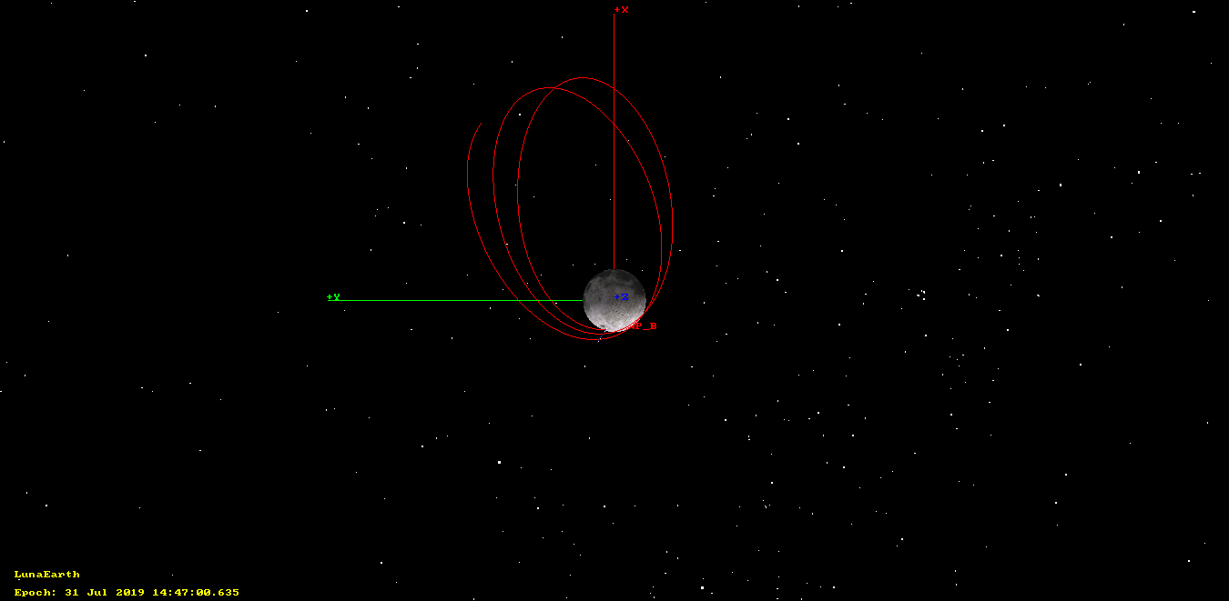
The figure below shows the orbit of DSLWP-B between July 28 12:00 UTC and the moment of impact, on July 13 14:47 UTC. The orbital state used for DSLWP-B is the 20190426 tracking file from dslwp_dev. The reference frame is arranged so that the +X axis points towards the Earth, and the Y axis lies on the Earth-Moon orbital plane. As we can see, unfortunately, the impact will happen on the far side of the Moon, where it is not observable from Earth.

However, it is possible to arrange a manoeuvre to modify the orbit slightly and make the impact point fall on the near side of the Moon, where it is visible from Earth. In the previous post we observed that, ignoring the collision with the lunar surface, the periapsis radius would continue to decrease after July 31, until reaching a minimum value in January 2020.

Therefore, it is possible to raise the periapsis radius slightly in order to delay the collision approximately half a lunar month, so that the periapsis faces the Earth at the moment of impact. The delta-v required to make this manoeuvre is small, as the adjustment to the orbit is subtle.

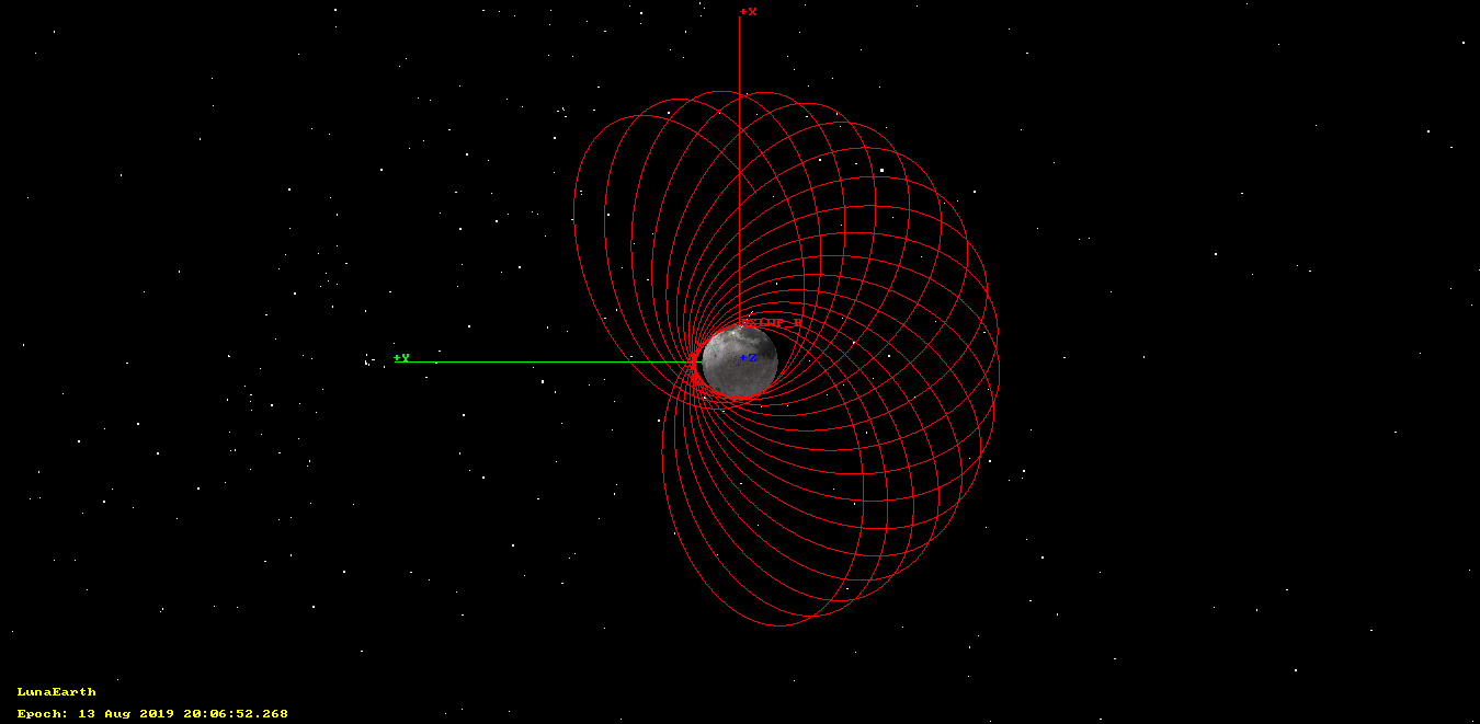
For instance, performing a prograde burn of 7m/s at the first apoapsis after July 1 delays the collision until August 13, producing an impact in the near side of the Moon. The resulting orbit can be seen in the figure below, which shows the path of DSLWP-B between July 28 and the moment of impact.

Adjusting the delta-v more precisely would make it possible even to control the time of the impact, so as to guarantee that the Moon will be in view of the groundstations at China and The Netherlands when the collision happens. However, this adjustment requires a very precise delta-v and is quite sensitive to the orbital state, so perhaps it is not feasible without performing a precise orbit determination and maybe some smaller correction manoeuvres following the periapsis raise.

Another possible problem that can affect the prediction of the impact point are the perturbations of the orbit caused by the lunar mascons, which can be noticeable when the altitude of the orbit starts getting small, and which haven’t been considered very carefully in this simulation (the non-spherical gravity of the Moon was only simulated up to degree and order 10).

The GMAT script used for this post can be found here.

On April 28, I got together with a few Spanish radio Amateurs to perform some experiments. One of the things we did was an angle of arrival experiment in the 145MHz Amateur band. The ultimate goal of the experiment was to be able to measure the angle of arrival of meteor reflections of the GRAVES radar at 143.05MHz. However, we also recorded a few other signals, such as the Amateur satellite band at 145.9MHz (intended to perform calibration of the setup) and the APRS terrestrial signals at 144.8MHz.

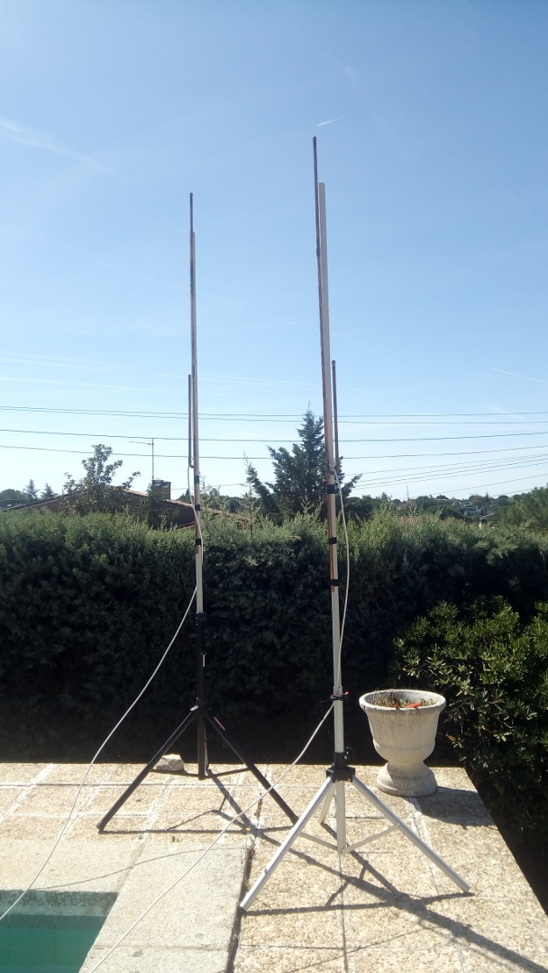
The antennas used in the experiment can be seen in the figure below. They are a pair of J-pole antennas built with copper pipe. The supports are PVC pipes. The antenna spacing is 1/2 wavelength at 143.05MHz. A run of around 15m of 75 Ohm TV coaxial cable is used to connect each antenna to the receiver.

This setup is less than ideal. The J-pole antennas were quickly built for the experiment, their impedance wasn’t measured, and using 75 Ohm coax is not optimal. However, they worked fine for strong signals. Also, the receiving location is not ideal. As it can be seen in the image, it is a suburban location with low buildings, so many of the signals arrive with multipath or in a non-line-of-sight manner.

The receiver is a LimeSDR. Its two channels are used to receive coherently from both antennas, so that the phase difference of the signals can be measured easily, in order to determine the angle of arrival. The spacing of 1/2 wavelength for the antennas was chosen to prevent the phase ambiguities that appear with a larger spacing.

The antenna baseline was laid so that the line perpendicular to the baseline had an orientation of approximately 35º. The antenna due northwest (right antenna in the figure above) was connected to the first channel of the LimeSDR, while the antenna due southeast was connected to the second channel.

The LimeSDR was set to a centre frequency of 145MHz and a sample rate of 5MHz. The LNAL input was used for both antennas, with an LNA gain of 30dB, TIA gain of 12dB, and PGA of 0dB. In order to save disk space, the following sub-bands of the full 5MHz of bandwidth were selected and recorded as IQ samples using 32bit floats:

• APRS: 144.800MHz, 25ksps
• GRAVES: 143.050MHz, 5ksps
• Satellites: 145.900MHz, 250ksps

The recording was made with the following GNU Radio flowgraph. The time span of the recording was from 09:48:40 UTC to 10:52:30 UTC. The recording files can be found here, together with a description of the recording format.

Satellites

The main interest of recording the 145MHz Amateur satellite band was to have a means of calibrating the setup and being able to determine the phase difference caused by the difference in feed line length to each antenna, as well as obtaining a more precise measurement of the antenna separation and the baseline orientation.

In theory, since the angle of arrival of a satellite signal can be computed from its TLE parameters, it is possible to compare this calculation with the measurements in order to determine the unknown parameters of the antenna array. An ideal signal for this is a line-of-sight signal that sweeps a large range of angles of arrival, so low Earth orbit satellite passes can be used as calibrators.

The satellite Nayif-1, which had a pass at 10:09 UTC was an ideal opportunity, since it transmits continuously a 1k2 BPSK telemetry signal at 145.940MHz.

This GNU Radio flowgraph was used to filter 10kHz of spectrum centred at 145.940MHz and to separate both channels for easier processing. The signal is then cross-correlated and analyzed in the following Jupyter notebook.

The position of Nayif-1 in the sky can be seen in the figure below. The azimuth sweeps a large range of angles of arrival, but unfortunately the elevation is not very high. This, together with the terrain obstructions around the antennas gave problems with multipath and non-line-of-sight signals, as we will see.

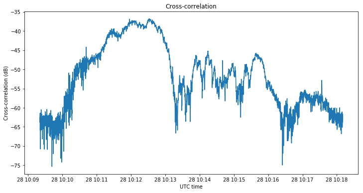
The magnitude of the cross-correlation is seen below. A coherent integration period of 100ms has been used in the correlation. The noise floor is seen in the left part of the graph to be at around -63dB. In the first minutes of the pass the signal is quite good, reaching up to 25dB SNR in cross-correlation. However, after 10:13, the signal presents deep fading typical of a Rayleigh channel.

The next figure shows the signal power received in each of the antennas. The power measured by antenna 2 has been increased by 5dB in the plot, because for some unknown reason the second channel showed less signal level than the first channel. We can see that the power at each antenna follows a different pattern, especially after 10:13 UTC. This is spatial diversity, which indicates multipath caused by nearby objects.

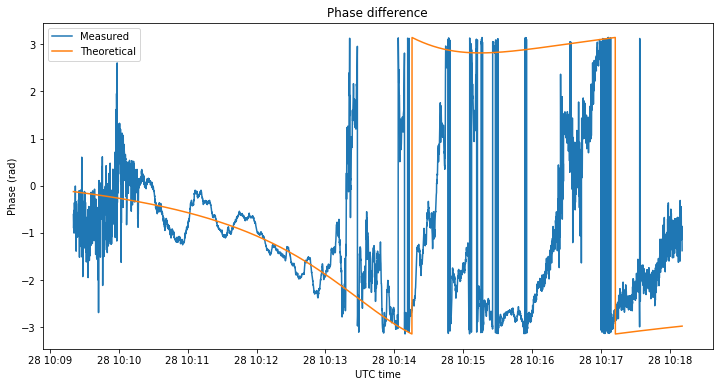
The figure below shows the comparison between the measured and the theoretical phase difference between each of the channels. The theoretical value has been obtained from the azimuth and elevation shown above, assuming a baseline orientation of 35º and length of 1/2 wavelength, and it has been adjusted vertically by hand to compensate for the phase difference between channels due to the difference in feed lines.

We can see that between 10:10 and 10:13 the measurements track approximately the theoretical value, although large excursions can be seen. This means that the signal is arriving with a certain degree of multipath rather than in a pure line-of-sight manner. After 10:13, the measurements no longer resemble the theoretical value at all, indicating that the signal is now arriving completely by non-line-of-sight.

Unfortunately, the multipath effects in the observation of Nayif-1 make it impossible to use this measurements to calibrate the antenna array.

APRS

In the recording there are APRS signals from several terrestrial stations. However, only the signals from ED4ZAE-3 are strong enough to be decoded. I wasn’t able to decode the signals from the remaining stations using Direwolf, so I don’t know their locations.

The calibration information about the phase difference due to different feedlines cannot be easily translated from 145.94MHz to 144.8MHz, so a new calibration has been made for APRS. Assuming a baseline orientation of 35º and length of 1/2 wavelength as above, the phase difference has been calibrated taking into account that the signals from ED4ZAE-3 should arrive from 237º, which is the straight line direction to the station. Note that this is only an approximate calibration. The phase difference of the signals from ED4ZAE-3 varies around 10º due to multipath propagation.

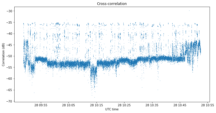
The figure below shows the cross-correlation magnitude in dB. The noise floor is between -55dB and -50dB, due to varying levels of interference. We have signals as strong as -35dB. As above, the coherent integration period for the correlation is 100ms.

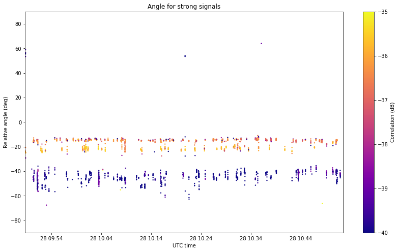
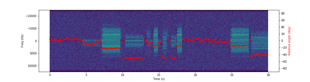
Below we show the angle measurements obtained for signals stronger than -41dB (this is made to filter out time intervals where no APRS packet was transmitted). The angle is shown as a relative angle to the baseline direction (35º). Therefore, an angle of -20º corresponds to an azimuth of 15º or 235º. Note that the radiation pattern for a phased array consisting of only two antennas is always symmetric with respect to the baseline, so such an array is unable to distinguish between angles of arrival which are symmetric with respect to the baseline.

The strength of the signals is color-coded as shown on the right of the graph. We see that the strongest signals, in yellow, which correspond to ED4ZAE-4, arrive from a relative angle of around -22º, as marked by the calibration. There is another station at around -15º which is slightly weaker than ED4ZAE-4, and some other station or stations between -40º and -50º. In this last case, the signals are weaker and the angles of arrival vary much more, probably due to greater multipath. It is also interesting to note that all the signals arrive from a relatively small interval of directions between -60º and -10º.

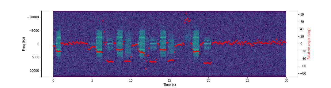
The two figures below show a couple of small excerpts from the recording. The spectrum is shown to aid identifying the different stations by their different strength and different modulation pattern (most likely caused by different FM deviations). The angle of arrival is shown using red dots. It is interesting to see how the different stations can be identified according to their angle of arrival. It is also interesting to note that the noise floor comes mostly from a well defined direction.

The analysis of APRS signals has been done in this Jupyter notebook.

GRAVES

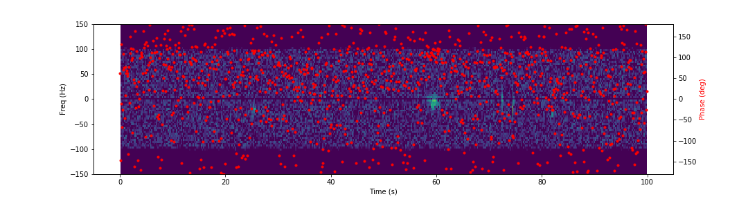
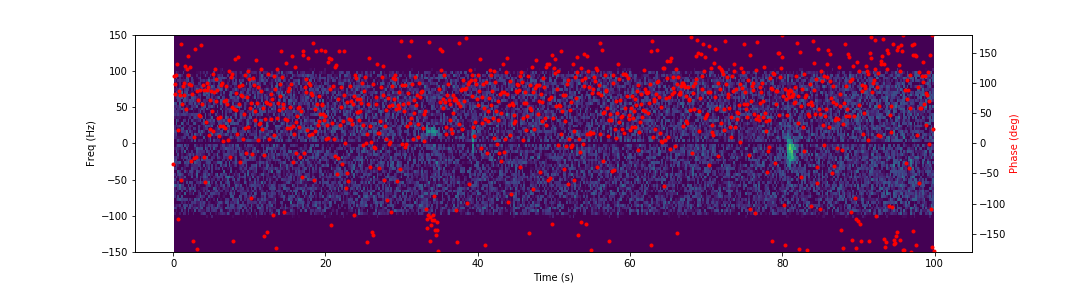
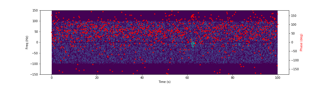
In the case of meteor scatter pings from GRAVES, the results are not very good. The recording has been filtered down to 200Hz of bandwidth and 1ksps using this GNU Radio flowgraph. The same kind of plot as for the APRS signals has been done, but without calibrating the phase offset, so the measures are phase differences instead of angles of arrival. This was done in the following Jupyter notebook.

Some of the most interesting excerpts from the recording are shown below. In comparison to the APRS excerpts shown above, the noise floor doesn’t come from any specific direction, as is to be expected if there is no noticeable interference.

Only the strongest and longest meteor scatter bursts produce phase difference measurements that are distinguishable from background noise, and even so, the quality of these measurements is not so good. Moreover, the phase differences corresponding to different bursts are completely different. This may be caused by the signals arriving by heavy multipath because of obstacles in the direction to GRAVES.

The array baseline was oriented perpendicularly towards GRAVES, so as to give the best sensitivity in measuring angles from the direction of GRAVES. However, that direction was blocked by low houses.

From the analysis of these results, it seems that to measure the angle of arrival of GRAVES pings successfully it is very important to have a clear view to the horizon. Also, using small yagis instead of omnidirectional antennas might help. If an observation using a baseline of 1/2 wavelengths such as in this experiment is able to determine that the angles of arrivals of GRAVES pings are all confined to a small range of azimuths, it is recommended to perform a second observation using a longer baseline, so as to obtain a greater sensitivity in the determination of the angles of arrival.

I would like to thank Luis Bernal EA5IDN, Gonzalo Carracedo EA1IYR, and Esteban Dauksis for their great help in the preparation and performance of this experiment.

A few days ago, I spoke about the future impact of DSLWP-B on the lunar surface, which will happen in the far side of the Moon around the end of July, and how the spacecraft could be manoeuvred to make the impact point fall on the near side of the Moon instead, so that it can be observed from Earth.

Philip Stooke made a very good remark in the comments saying that the impact might have been planned on the far side of the Moon deliberately in order to avoid Apollo landing sites and other heritage sites. This is a very valid concern. By all means, the crash should be planned to avoid disturbing heritage sites or other areas of specific interest.

It is easy to compute in GMAT the location of the impact point. Using the 7m/s prograde burn that I proposed, we obtain the following.

The exact location of the impact is 25.8098º of latitude and -1.7261º of longitude. This is located in Palus Putredinis. The map of the Apollo sites can be browsed in Google Moon, and Wikipedia has a more complete map including Russian and Chinese landings. The nearest heritage site to the impact point is Apollo 15, at 26.1322°N 3.6339°E. The separation between both sites is approximately 150km. This is relatively small if we consider that the Moon radius is 1737km and that there are only a dozen historical sites scattered over the near side.

I have tried to modify the delta-v of the manoeuvre to change the impact point. With careful planning it should be possible to put the impact point well away from any heritage site. However, this is not so easy to do. If we look at the figure below, which appeared in this post, we can understand why.

If we raise or lower the periapsis radius slightly, the impact date only changes by a few days. This makes the impact point fall nearby, since the Moon has not rotated much in these few days. If we raise the periapsis radius enough, then the impact date is delayed to the next local minimum of the curve, which happens in approximately half a lunar month. In this time, the Moon has rotated half a turn, so the impact point falls on the opposite side of the Moon.

This is the technique that I used when I proposed the manouvre to delay the impact until mid August and make the impact point fall on the near side of the Moon. However, we don’t have much freedom to adjust the longitude of the impact point to make it fall further from Apollo 15. If we increase the delta-v slightly, then the impact point is close by. If we increase it more, then the impact point is delayed to late August so that it falls on the far side.

In any case, I think that 150km of clearance from the Apollo 15 site is enough, provided that the necessary precision can be guaranteed both in the determination of the orbital state (an error in the right ascension of the ascending node could make the impact point fall dangerously close to Apollo 15) and the delta-v. This is something that will require the feedback from the operators of the satellite, if they are interested in making this kind of manoeuvre.

The first Amateur VLBI experiment with DSLWP-B was performed on 2018-06-10. In that experiment, the 250baud GMSK beacons at 435.4MHz and 436.4MHz were recorded in the 25m PI9CAM radiotelescope in Dwingeloo, The Netherlands, and a 12m repurposed Inmarsat C-band dish in Shahe, Beijing. These synchronized recordings were processed later to obtain delta-range and delta-velocity measurements. Due to the low baudrate, the noise of the delta-range measurements was quite high, on the order of 20km. Since the beacons were short transmissions of 15 seconds, making accumulated phase measurements was not possible.

Another Amateur VLBI experiment was performed on 2018-11-21. The novelty of this experiment was that 500baud GMSK SSDV transmissions were made on 436.4MHz. These long transmissions, lasting around 30 minutes each, allow us to make accumulated phase measurements. Also, the higher baudrate reduces the noise in the delta-range measurements. Another novelty was that a third station, the Harbin Institute of Technology Amateur Radio Club BY2HIT groundstation also joined the experiments, so observations from three stations are available.

This post is an account of the results I have obtained processing the observations from 2018-11-21.

Observation correlation

The observations of the three groundstations can be downloaded from the file repository of CAMRAS (search for 2018-11-21). The format of these files is the GNU Radio metadata format, with 32 bit float IQ samples and 40ksps. The first step in processing these files is to use convert_metadata_file.py to convert the files to complex64 IQ files, removing the metadata. This makes it easier to process the files with NumPy later.

The next step is to take note of the timestamp corresponding to the start of each of the recordings. This is stored in the file metadata and can be read by using

gr_read_file_metadata $file | grep Seconds | head -n 1

The correlate_recordings.py script is the main piece of the pipeline for processing the observations. It reuses many signal processing blocks from my Moonbounce processing pipeline. The script runs on each baseline (i.e., on each pair of recordings) and performs the following tasks:

• Alignment of the recordings according to the timestamps
• Calculation of expected Doppler using GMAT
• Correction of expected Doppler on each observation
• Lowpass filtering of each observation
• Correlation in time and frequency using FFTs

The correlation algorithm is very similar to the one used in the first Amateur VLBI experiment, but the FFT size is \(2^{17}\) samples, or 3.2786s, so as to give a good balance between SNR and update rate of measurements.

All the results are saved to either NetCDF4 files using xarray or NPY files for later analysis.

The script needs to take into account the frequency offset of the transmitter on-board DSLWP-B, so as to correct this offset to bring the signal to baseband before lowpass filtering the observation. This offset was determined using the Moonbounce processing scripts to be -250Hz for the 436.4MHz transmitter. The 435.4MHz recordings have not been processed yet, since they are not so interesting, as they only contain short GMSK beacons.

Since the Python script takes a lot of parameters, the Bash script run.sh is used to run the script with the correct parameters on each of the recordings. The output files can be found here.

Observation postprocessing

The output files of the correlation script are loaded and processed in a Jupyter notebook to compute and evaluate the VLBI measurements. Besides the output files, two additional values are needed in this notebook. These values are printed out by the correlation script and stored in the log.

The first of them is the timestamp associated to the first sample in the correlation. This is computed by the correlation script because it can remove samples from the start and end of each observation in the baseline in order to line them up in time. The second is the residual clock offset. The correlation script tries to line up the two observations perfectly according to their respective timestamps, but it does so by shifting an integer number of samples. Therefore, a clock offset smaller than a sample period might remain after this step. This clock offset must be applied later in order to correct the measurements.

The postprocessing of the correlation outputs produces two types of measurements: delta-range measurements using time difference of arrival, and accumulated phase difference measurements. The accumulated phase differences also measure the delta-range, but they have an unknown offset, and are subject to other additional problems which I will explain later. However, phase measurements are much less noisy than the delta-range measurements, as they use the carrier phase, which is 436.4MHz, a much higher frequency than the 500baud modulation rate.

The accumulated phase differences can be differentiated in time to obtain delta-velocity measurements using the Doppler difference, as it was done in the first experiment. These are very accurate, since they are also derived from the carrier phase.

Measurements filtering

As it has been the case in previous Amateur VLBI experiments using low baudrate signals not intended for ranging, such as the first DSLWP experiment and the LilacSat-2 experiment, there is a huge gap between the precision of the measurements derived from time difference of arrival, such as the delta-range, and the phase difference, such as the delta-velocity. The error of the delta-range measurements is on the order of 10km, while the error in the delta-velocity measurements is on the order of 0.1m/s.

To try to bridge this gap, it is possible to use the delta-velocity measurements to smooth out or filter the delta-range measurements. Here I have tested two different smoothing algorithms to evaluate their performance.

The first of them is usually called the Hatch filter in the GNSS literature. If \(r_k\) and \(v_k\) are the delta-range and delta-velocity measurements respectively, we compute filtered delta-range measurements \(y_k\) as\[y_k = \alpha r_k + (1-\alpha) (y_{k-1} + v_k),\]where \(\alpha > 0\) is a small parameter. Thus, we see that the Hatch filter is just a weighted average between the current non-smoothed delta-range and the previous smoothed delta-range propagated using the delta-velocity.

For very small values of \(\alpha\) the filter gives out a very smooth output, but it might drift from the true value, since errors in the propagation using the velocity accumulate. For larger values of \(\alpha\) the output is not so smooth but it follows the measurements \(r_k\) more closely.

The second method I’ve used is the Kalman filter. The model on which this filter is based considers a state \(x_k\) which evolves linearly with some stochastic perturbations as\[x_{k+1} = F x_k + n_k,\]where \(n_k\) is known as the process noise and is Gaussian with covariance \(Q\). The state is observed linearly, with some measurement noise, to produce observations\[z_k = Hx_k + m_k,\]where the measurement noise \(m_k\) is Gaussian with covariance \(R_k\).

The Kalman filter is an optimal estimator for the state \(x_k\) and the state error covariance \(P_k\) given a series of measurements \(z_k\) and their error covariances \(R_k\).

In our case, we consider a really simple model where the state is \(x_k = (r_k, v_k)^T\), the measurement matrix is \(H = I_{2\times 2}\), the state evolution is\[F = \begin{pmatrix}1 & 1\\ 0 & 1\end{pmatrix},\] and \(Q\) and \(R_k\) are diagonal matrices.

Correction of clock jumps

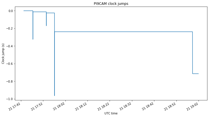
The PI9CAM recordings have clock jumps, probably caused by lost samples while the recording was made. However, since the GNU Radio metadata file format saves timestamps periodically, it is easy to compute and correct these clock jumps. The figure below shows the jumps in the clock of the PI9CAM recording. These are corrected in the correlation postprocessing, by adding the clock offset to the computed delta-range.

Evaluation of the measurements

After obtaining the measurements, the Jupyter notebook is used to plot and evaluate them. The figure below shows the amplitude of each of the correlations.

We can see that each of the baselines has a different time span, since PI9CAM joined the experiment late and Harbin finished earlier. The short spikes correspond to GMSK telemetry beacons, while the long periods when the signal is transmitting correspond to SSDV image downlinks. We see that the SNR on the PI9CAM-Shahe and PI9CAM-Harbin baselines is an excellent 40dB, while the SNR on the Shahe-Harbin baseline is only 20dB. This gives lower quality measurements, but the measurements for the Shahe-Harbin baseline can also be obtained by subtracting the PI9CAM-Harbin and PICAM-Shahe baselines, thus obtaining lower noise measurements than if using this baseline directly.

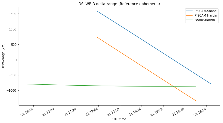
According to the GMAT ephemeris, the delta-range measurements on each of the three baselines should evolve as shown in the figure below.

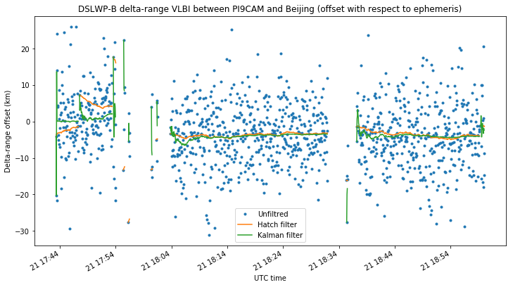
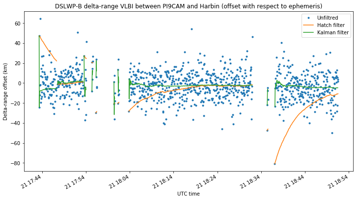
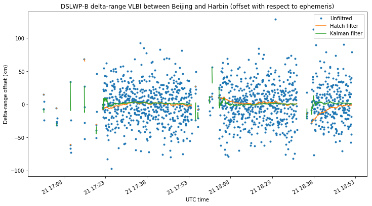
The three figures below show, for each baseline, the offset between the delta-range VLBI measurements and the GMAT reference ephemeris. Unfiltered, Hatch filtered and Kalman filtered measurements are compared.

The jumps in the filtered measurements during the first SSDV transmission on the PI9CAM baselines are caused by one of the PI9CAM clock jumps. The filters are reset at the clock jump due to unavailability of measurements during the clock jump.

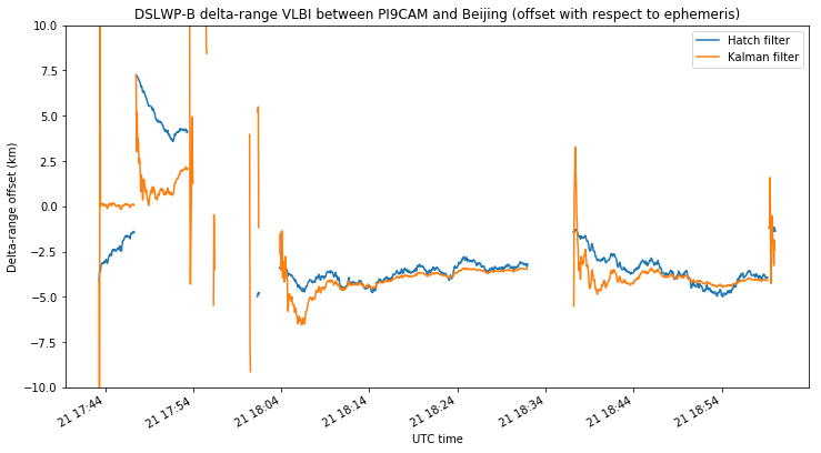
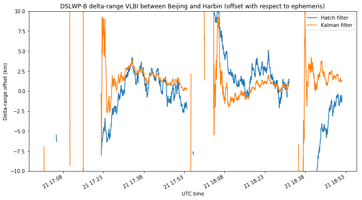
We see that the delta-range noise in the unfiltered measurements for the PI9CAM baselines is around 10-20km. On the Shahe-Harbin baseline it is on the order of 50km, due to the much lower SNR. The noise of the filtered measurements is much lower, so we plot them below without the unfiltered measurements to examine them in more detail. The three plots use the same vertical axis to ease comparisons.

These plots illustrate the main difference between the simple Hatch filter and the more complex Kalman filter. The Hatch filter doesn’t have memory, and performs in the same manner during the course of an observation. This makes adjusting the parameter \(\alpha\) tricky. Too small and the filter will take a lot of time to converge to the correct value, as it happens in some of the plots above if the filter was started with a delta-range measurement with a large error. Too large and the filter will be very noisy.

On the other hand, the Kalman filter propagates the covariance of the state error \(P_k\) and uses it to vary the smoothing as time progresses. In the beginning of each transmission, the filter doesn’t have a good estimate of the state \(x_k\), so it tries to move quickly to converge to a good estimate, giving a noisier output. As the transmission goes on, the filter gains confidence in its estimate of the state \(x_k\), reducing the noise in its output at the expense of responding more slowly to unexpected jumps in the state.

We see that, for the PI9CAM baselines, the noise of the Kalman filter is very small in comparison with the unfiltered delta-range measurements, perhaps on the order of 100m. On the other hand, the Shahe-Harbin baseline gives a noise of around 1km, owing to the much lower SNR.

There seems to be a bias of around -5km, -2.5km and 2.5km in the delta-range measurements of each baseline respectively. This is probably caused by errors in the reference ephemeris used in GMAT. However, it is convenient to note that in comparing the VLBI measurements with the GMAT ephemeris we are using a simple model that ignores the finite propagation speed of light. It is assumed that the delta-range at time \(t\) is given by\[\|s(t) – g_1(t)\| – \|s(t) – g_2(t)\|,\]where \(s\), \(g_1\) and \(g_2\) denote the position of the satellite, first groundstation and second groundstation respectively. However, in reality, the delta-range at time \(t\) is given by the more complicated formula\[\|s(t-\tau_1(t)) – g_1(t)\| – \|s(t-\tau_2(t)) – g_2(t)\|,\]where the propagation delays \(\tau_j\) satisfy\[c\tau_j(t) = \|s(t-\tau_j(t)) – g_j(t)\|.\]

Phase measurements

As I have already mentioned, phase difference measurements give very good precision, as they use the relatively high carrier frequency to measure delay, instead of using the low baudrate modulation. However, they have several associated problems that need to be treated carefully.

First of all, phase difference measurements have an ambiguity or offset. In the ideal case when the local oscillators of the two stations participating in the baseline are perfectly synchronized, this offset is an integer number of cycles which is caused by the fact that the phase can only be measured modulo one cycle. Performing accumulated phase measurements, i.e., relating a phase measurement with the measurement of the previous epoch allows us to have a common offset for the complete sequence of measurements, instead of having a different and unrelated offset per measurement. If one wants to give physical meaning (as delta-ranges) to the phase difference measurements, this unknown integer number of cycles needs to be determined.

However, usually the local oscillators in the groundstations are synthesized using PLLs, and these can lock to a different phase offset every time they are started. In practice, this means that the local oscillators of the two groundstations participating in the baseline are not synchronized, but rather have an unknown and fixed offset. The consequence is that the offset for the accumulated phase measurements is no longer an integer, but any value. Therefore, it cannot be determined exactly, but only approximated.

The usual procedures for determining the phase offset involve filtering delta-range measurements based on the modulation, which are unbiased. If the noise of these measurements can be reduced to less than one wavelength, then an integer phase offset can be determined exactly. In the case of DSLWP-B, the difference in precision of the modulation-based and phase-based measurements is so large that it is probably impossible to use this kind of procedures.

Another problem regarding phase measurements is errors in the frequency of the transmitter. Indeed, if the nominal frequency of the transmitter is \(f\), an error of \(\delta f\) will cause an error in the determination of velocity of\[\delta v = v \frac{\delta f}{f}.\]Integrating this error over a time interval \(0 \leq t \leq T\) produces an error in delta-range of\[\delta r = (r(T)-r(0))\frac{\delta f}{f}.\]

In the case of DSLWP-B, the change in delta-range over the course of an observation is on the order of \(10^6\)m. Therefore, a frequency error of 1ppm (which is a good assumption for the DSLWP-B TCXO) produces an accumulated error of 1m at the end of the observation. This is small in comparison with other sources of error, so this kind of errors can be ignored.

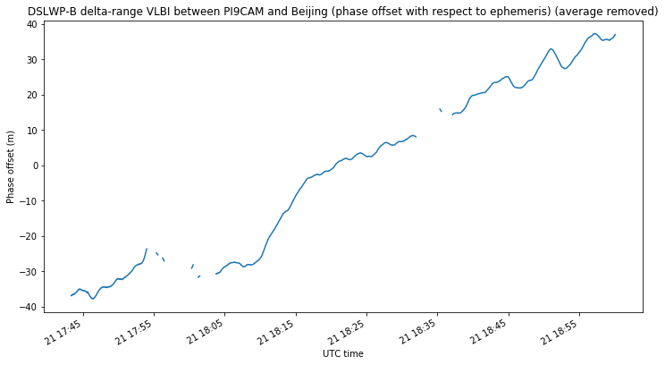
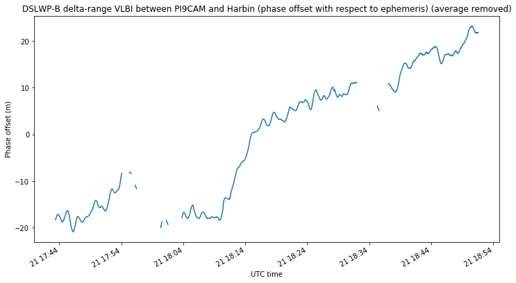
In any case, the performance of the phase difference measurements can be evaluated by plotting the diference between the delta-range obtained from these measurements and the reference ephemeris. The average needs to be subtracted, so as to remove the unknown offset in the accumulated phase. This is shown in the figures below.

We can see that the noise of the phase measurements is sub-metric, as is to be expected. An error of several tens of metres accumulates with time. This is most likely due to small errors in the reference ephemeris.

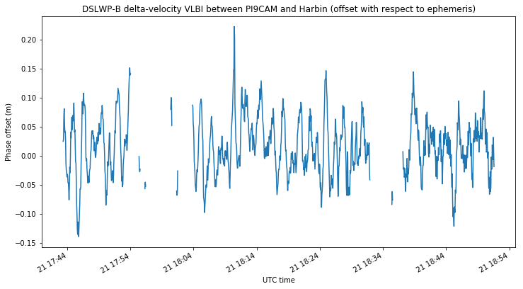
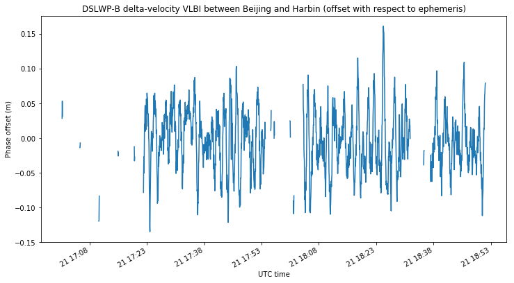
It is also noticeable that the phase measurements show some kind of wavy pattern. This is best seen in the delta-velocity measurements, which are the time derivative of the plots shown above.

The cause of this oscillating error is not known. It might even be caused by errors in the frequency references of the groundstations. Even though each groundstation uses a GPSDO, the frequency reference can have some small errors, since a GPSDO works by estimating the phase error of a voltage-controlled oscillator and steering it to phase-lock it to GPS time. The error seen in the figures above corresponds to a reference frequency error of 0.2ppb, which is perfectly compatible with the steering error of a GPSDO.

Conclusions

We have seen that the error in delta-range measurements using time of arrival measurements is large, on the order of 10km, due to the low baudrate modulation used for the VLBI experiment. On the other hand, measurements derived from observing the carrier phase have an error of sub-metric level. It doesn’t seem possible to bridge this gap of 4 orders of magnitude and use unbiased delta-range measurements to remove the inherent biases in phase-based observations.

The use of simultaneous carrier phase observations on 435.4MHz and 436.4MHz would provide a 1MHz signal to obtain estimations having an error of metric or decametric level and ambiguity of an integer number of 300m wavelengths. Therefore, it might be possible to use a tiered approach where unbiased modulation-based observations are used to compute the unknown integer number of cycles for the 1MHz signal, and the relatively low noise of the (now bias free) 1MHz signal is used to obtain unbiased carrier phase based measures. This would require simultaneous long transmissions in both bands, but this hasn’t been performed so far due to concerns of overheating in the transmitter.

There are some unknown biases present between the observations and the reference ephemeris. While an error in the ephemeris can explain these completely, instrumental biases or other biases in the signal processing chain shouldn’t be ruled out completely. These Amateur VLBI groundstations haven’t been commissioned by performing calibration observations, with sources such as a satellite for which precise ephemeris are available. The use of a more complex model for the interpretation of delta-ranges, including the finite propagation speed of light effects would also be a useful exercise.

Finally, the ultimate goal of these observations is to perform precise orbit determination with them. No such attempts have been made yet. Trying to fit an orbital state vector to the observations would serve as additional validation of the observations, ruling out possible errors in the published ephemeris. However, it is convenient to note that the observations analyzed in this post last only a 2 hour activation period of DSLWP-B. To perform accurate orbit determination, observations need to be made at well spaced points along the orbit. The orbital period of DSLWP-B is around 20 hours. Therefore, well spaced activations and observations on the same day or on nearby days should be planned to perform this task. This also makes observation planning tricky due to the requirement of a common window on the longer Europe-China baselines.

Last Sunday, Julián Fernández EA4HCD, released a high altitude balloon carrying a LoRa payload as a preliminary test for the FossaSat-1 pocketqube that he is devolping with Fossa Systems. You can see a video of the release in this tweet. The balloon was launched near Madrid, and burst at an altitude of approximately 24km, having travelled some 180km southeast.

The payload had two transmitters: An SX1278 LoRa transceiver transmitting at 434.5MHz with 10mW alternating between LoRa and RTTY, and an 868MHz 25mW LoRa transceiver that was received on The Things Network. Simple groundplane 1/4-wave monopole antennas were used.

I went to the countryside just outside my city, Tres Cantos, and set up a station to record the transmissions on 434.5MHz. The station consisted of a 7 element yagi by Arrow Antennas, set in vertical polarization and placed on a camera tripod on the roof of my car, and a FUNcube Dongle Pro+. This is a brief analysis of the recording.

I was able to receive the signal from the balloon since shortly after launch, at 15:37 UTC, until 18:45 UTC, when I took the station down. The balloon burst a few minutes before 19:00 UTC, and the payload quickly descended to ground, as it had no parachute. The recording was made at 192ksps with a centre frequency of 434.5MHz. At some point I changed the centre frequency to 434.502MHz because the RTTY signal went too close to the FUNcube Dongle centre spur due to the transmitter’s frequency drift.

The recording can be downloaded from this Zenodo publication. It is in Linrad raw file format. It can be read as a little-endian int16 IQ file by skipping a 41-byte header at the beginning of the file.

The figure below shows the spectrum of a segment of the recording in Linrad. Approximately every 30 seconds a LoRa beacon was transmitted followed by an RTTY beacon. The mode used by LoRa was SF11 125kHz, while RTTY used 240Hz of shift, 45 baud, 7bit ASCII, and 1 stop bit. There are also moderate levels of interference, formed by wideband interference and some narrowband interference around 434.525MHz. I do not know the sources of this interference.

The figure below shows a detail of the LoRa beacon in Inspectrum. The characteristic chirp modulation is visible. Also, the wideband interference is seen to have a pulsed pattern.

The RTTY signal was decoded in real time using fldigi. The payload transmitted its latitude and longitude, obtained from a uBlox M6 GPS, its height, obtained from a BMP280 barometer, and the temperature. I used the position data to aim the antenna. Unfortunately, the GPS stopped updating its position above 18km of altitude, due to CoCom limitations. The signal had a lot of frequency drift, making decoding RTTY quite tricky.

Julián tells me that he was unable to decode the LoRa transmissions at 434.5MHz due to the frequency drift. On the other hand, several gateways from The Things Network received the 868MHz LoRa transmissions, so perhaps this transmitter used a better oscillator, or the SF7 125kHz mode used in 868MHz tolerates drift better.

I have tried to decode the LoRa beacons in the recording with gr-lora, but so far I haven’t obtained anything. Probably it is due to the frequency drift, or maybe due to a not so good support of the SF11 mode in gr-lora.

I have also processed the recording to compute estimates for the power of the LoRa and RTTY signals. The RTTY power is simple to compute: I have used the signal plus noise power in 5kHz bandwidth, in order to be able to ignore the transmitter drift. For LoRa, I have used the following signal processing.

First, the signal is dechirped assuming an upchirp. To do so, I have used something which I would call the IQ equivalent of a Shepard tone. This is a signal with continuous phase and frequency and such that its frequency always increases at a constant rate. Of course it is possible to do this without quickly overflowing things due to aliasing: once the frequency gets to \(f_s/2\), it aliases back to \(-f_s/2\), so in reality the frequency we are generating is a saw-tooth between \(-f_s/2\) and \(f_s/2\) (here \(f_s\) denotes the sample rate).

The more conventional way of performing dechirping would be to replicate what the transmitter is doing and generate a chrip whose frequency is a saw-tooth between -62.5kHz and 62.5kHz. The problem with this is that, unless this chirp is aligned in time with the LoRa signal, the LoRa chirps will break into two tones at different frequencies due to the frequency jump of the dechirping signal (see my post about dechirping CODAR for more information).

The Shepard tone doesn’t require alignment and it never breaks the LoRa chirps into two tones, since it has continuous frequency and phase. One disadvantage of the Shepard tone is that it places each of the 10 upchirps forming the LoRa preamble at a different frequency, while the more conventional method puts them in the same frequency.

To generate this Shepard tone, we must know the slew rate, or chirp rate, of the LoRa chirps. A LoRa mode has two main parameters, the spreading factor \(S\) and the bandwidth \(B\). The duration of each chirp is \(B/2^S\), and each chirp covers a bandwidth \(B\), increasing from \(-B/2\) to \(B/2\). Thus, the slew rate is \(B^2/2^S\). In our case, we have \(S = 11\) and \(B = 125kHz\), so the slew rate is approximately 7.6MHz/s.

The LoRa signal dechirped with the Shepard tone is shown in the figure below. Note the 10 tones corresponding to the 10 preamble upchirps.

After dechirping, a 1024 point FFT is computed. At a sample rate of 192ksps, this gives us an FFT length of 5.3ms. Since the duration of each chirp is 16.4ms, the dechirped tones occupy several FFT windows, so at least some FFT windows are guaranteed to be filled completely with a dechirped tone, regardless of temporal alignment. The maximum amplitude among all the FFT bins is taken as the estimate of the LoRa signal power.

The GNU Radio implementation of this algorithm is shown in the figure below. The LoRa signal comes from the top.

This kind of algorithm works well for estimating the LoRa signal power during the 10 preamble upchirps, ignores the two downchirps marking the end of the preamble, and works moderately well during the data despite the frequency shifts, since the FFT windows are shorter than a complete chirp. In fact, the figure above shows that there are still many relatively long dechirped tones during the data section.

The output of this algorithm is then averaged in segments of 300 FFTs, or 1.6 seconds. This guarantees that at least one averaging window is completely occupied by a LoRa packet, regardless of synchronization.

The results of these power estimators are shown below, comparing the LoRa and RTTY signals. Of course, both follow a very similar behaviour, since they use the same transmitter and antenna.

It would be interesting to plot signal power against distance. According to free space path loss, we should see an inverse square law dependence between power and distance.

The plots for this post have been done in this Jupyter notebook. The signal processing has been done in this GNU Radio flowgraph. To run the flowgraph, a FIFO is first created using

mkfifo /tmp/sonda.fifo

and then the recording is sent through the FIFO skipping the header by doing

tail -c +42 recording.raw > /tmp/sonda.fifo

This allows us to read the recording directly in GNU Radio as an int16 IQ file.

A month ago, I spoke about planning the passes of the Moon through the beam of my QO-100 station. These give an occasion to observe the Moon without moving a dish that is pointing to Es’hail 2. The next opportunity after writing that post was on May 16 at 20:16 UTC.

Since I wasn’t going to be at home at that time, I programmed my computer to make a recording for later analysis. I recorded 4MHz of spectrum centred at 10367.5MHz using a LimeSDR connected to the LNB that I use to receive QO-100. The recording was planned to be 30 minutes long starting at 20:01 UTC, but for some reason only approximately 27 minutes were recorded.

This kind of events can be used to measure Moon noise and receive 10GHz EME signals. This post is an analysis of my recording, looking at these two things.

The Moon noise measurement was done at 10366.5MHz with 1MHz of bandwidth, in order to avoid the LimeSDR centre spur and any possible signals at 10368MHz. GNU Radio was used to filter this chunk of spectrum and perform average power measurements, taking one power reading per second.

The power readings were analyzed in a Jupyter notebook. The figure below shows the noise compared with the separation of the Moon from the centre of the dish (assuming that it is pointing perfectly well to Es’hail 2).

We note that the noise decreases almost 0.2dB in the first 10 minutes of the recording. This is caused by the change in temperature of the LimeSDR as it starts receiving and streaming samples. The LimeSDR had been connected to the computer by USB for a long time before the recording started, but it wasn’t streaming samples. This is a lesson I’ve learned: it is important that the receiver is completely functional for a long time before the start of the recording, so that it has a stable temperature.

It is convenient to remark that many RF active components have a gain that varies noticeably with temperature and other factors. These gain variations place a practical limit to long Amateur radioastronomy observations.

We see that there is a hump of approximately 0.05dB in the noise which coincides perfectly with the Moon passing through the beam of the dish. This is the Moon noise. After the Moon has passed through the dish, the noise varies somewhat erratically. I don’t know the reason for these variations.

The receiver used for this experiment was a 1.2m offset dish from diesl.es and an Avenger PLL321S-2 Ku-band LNB modified to use an external 27MHz reference. I would have expected a higher Moon noise from this station: between 0.1 and 0.15dB. Thus, I have spent some time trying to understand why I am getting a reduced performance.

One thing to be cautious of is the noise figure of the LNB. The measurements done by Ian Roberts ZS6BTE show that commercial Ku-band LNBs can have a rather high noise figure below 10.7GHz. To assess the performance of my LNB, I performed a Y-factor test a few days after the Moon observation. I used the LNB placed in the dish as cold measurement, and the LNB dismounted from the dish and pointing to the nadir as hot measurement.

I have obtained the following Y-factors depending on frequency: 2.5dB at 10366.5MHz, 3dB at 10488MHz, and 3.4dB at 10800MHz. The ambient temperature was 17ºC, so we take the hot source as 290K. For the cold source we use an educated guess of 70K (which is supposed to come mainly from dish spillover). Using these values we get noise figures of 2.4dB, 1.8dB and 1.4dB at the measurement frequencies.

Note that this is just a rough approximation, since an typical estimate was used for the cold temperature. Also, it is possible that the measurement of the Y-factor at 10800MHz is too low due to signals from the GEO satellites affecting the cold measurement, even though I tried to select a clear frequency for the measurement.

Using the VK3UM EME Calculator, a noise figure of 2.4dB, spillover of 70K, and a 1.2m dish with 40% efficiency yield a Moon noise of 0.11dB, which is noticeably more than the 0.5dB I have obtained.

Something we need to have in mind is that the Moon didn’t pass through the centre of the dish beam during the experiment. We can assume that the closest the Moon got to the centre of the dish is 0.5º. According to this calculator, a 1.2m dish can be between 0.5 and 1dB down at 0.5º off-beam depending on its efficiency. However, this decrease in gain would only account for a small difference in the Moon noise.

Therefore, I haven’t come up with a convincing explanation for the difference between the theory and my observations. It will be interesting to observe future passes of the Moon through the dish beam to see if I get different results.

Now we turn our attention to any possible EME signals present in the recording. The first signal to search is the DL0SHF EME 10GHz beacon, which transmits at 10368.025MHz every time that the Moon is visible from Germany. According to the VK3UM EME Planner, the Doppler between Germany and my station in Spain at the time the recording was made was 7.3kHz.

By looking at the recording using rfplot from strf (see this post for a tutorial), we find the signal at the expected time and frequency, as shown in the image below.

If you look at the figure above, perhaps you’ll notice something odd. The DL0SHF beacon is supposed to transmit FSK-CW on odd minutes and QRA64D on even minutes. The FSK-CW transmissions can be seen more clearly in the image, but it seems that there is an FSK-CW transmission every minute rather than every two minutes as expected.

At first I suspected that I messed up something with my recording (maybe the sample rate, or the sample format), but the shift between the FSK-CW tones is 400Hz, as expected, and the signals are visible between 20:14 and 20:20, which coincides with the period when the Moon passed through the dish beam and when the Moon noise hump was visible.

Therefore, I think it is very unlikely that I’ve messed something up with the recording, and somehow the beacon was transmitting “faster” than it should. I have asked some Spanish EME operators and they didn’t observe anything odd with the beacon, even on the same day that I performed the observation. Maybe this was a temporary problem of short duration.

Besides the DL0SHF beacon, I haven’t detected any other EME signals in the recording.

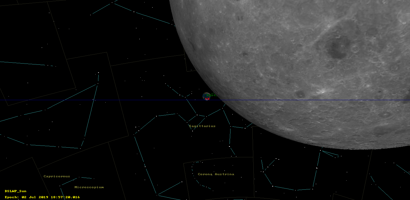
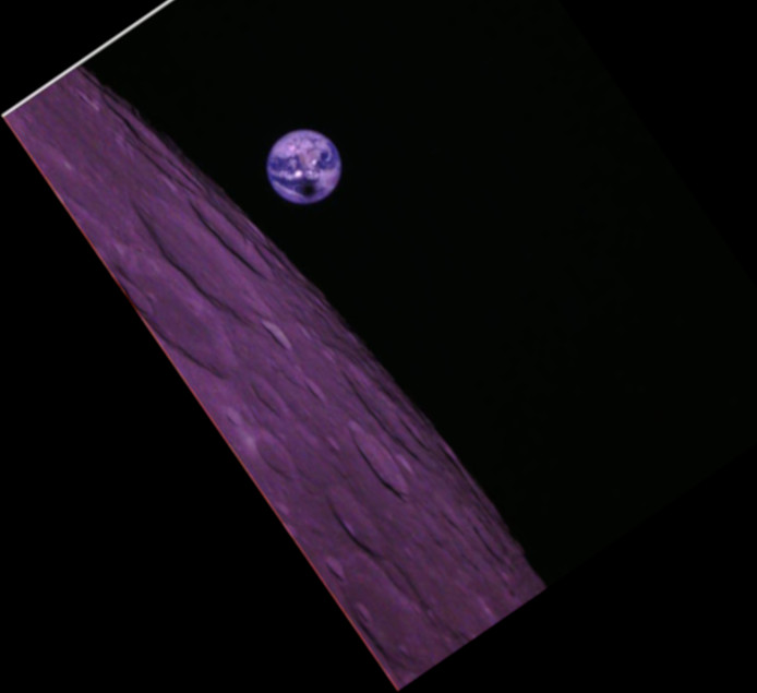
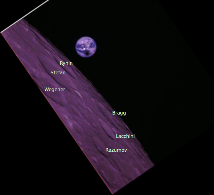
Yesterday, Wei Mingchuan BG2BHC sent an email to the team of DSLWP-B collaborators saying that the first week of June would give good opportunities both to take images of the Moon and Earth (as it has been done in other occasions) and to perform VLBI sessions involving Dwingeloo, Shahe, Harbin, and perhaps Wakayama University, which has a 12m dish. Here I show the preliminary plan proposed by Wei and a few graphs useful for camera and VLBI planning.

I have updated my camera planning Jupyter notebook to use the 20190603 ephemeris from dslwp_dev. The figure below shows the camera view.

Wei has proposed to activate the Amateur payload of DSLWP-B on 2019-06-03 03:05:00 UTC, taking a series of 9 images with 10 minutes of spacing, starting at the payload activation. As we can see in the figure above, this is the time when both the Earth and Moon are visible in the camera frame and nearest to the centre of the image, so it is the best occasion for taking images.

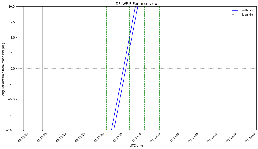
During the imaging session, the Earth will hide behind the Moon, giving the opportunity to take “Earthrise” pictures. The graph below, which I call an Earthrise view, shows the angular distance between the Earth and the lunar rim. This can be used to see when the Earth will be hidden behind the Moon. The imaging instants are marked with green lines. We see that there is good coverage of the Earthrise event, so a good animation can be made.

The Earth also hides behind the Moon on two other occasions. No pictures are planned to be taken during these, but the Earthrise plots are shown below for completeness. Note that from the point of view of the groundstations on Earth, these correspond to occultations of DSLWP-B behind the Moon, so they are also interesting for planning VLBI observations.

For planning VLBI observations, we need that DSLWP-B is in view of all the groundstations. We assume an elevation mask of 5º. I have made a VLBI planning Jupyter notebook to plot the elevation of DSLWP-B as seen from each of the groundstations and to mark the time windows when it is above 5º for all the groundstations. The plots are shown in the figures below. Each of them represents a single day.

The windows where the four groundstations are available for VLBI are shown in green, while the remaining time is shown in red. The observation times proposed by Wei are marked with red vertical lines. These are from 07:00 to 09:00 on June 4, 5 and 6, and from 08:00 to 10:00 on June 7.

We see that all the observation windows fall inside the VLBI window (except on June 3, when the activation will be used for imaging). The plan is to take the images on June 3 and then download the images from June 4 to June 7, taking advantage of the long SSDV transmissions to perform VLBI.

Another interesting aspect that I mentioned in my analysis of a previous VLBI experiment is that if VLBI is going to be used for orbit determination, it is desirable to perform observations at different points along the orbit. I have included in the graphs shown above the true anomaly of DSLWP-B as a purple dashed line. This can be used to see where is DSLWP-B in its orbit on each of the VLBI observations. Taking into account the four windows chosen for VLBI, we have an almost continuous coverage of true anomaly between 0 and 200º, which is pretty good.

As I have remarked above, 2019-06-04 00:00 and 2019-06-04 20:30 would also be interesting moments to perform VLBI, since they correspond to occulations of DSLWP-B behind the Moon. However, at 00:00, the Moon is not yet visible in Dwingelooo, so VLBI could only be performed with the much shorter baselines between East Asian stations. At 20:30 the groundstation coverage is rather poor: the Moon is only visible in Dwingeloo, and at a rather low elevation.

Keep in mind that the observation times shown in this post are still a proposal and need to be confirmed. In particular, it is not known if Wakayama will be able to participate in the observations, as they need to replace the feed in the dish. I will update the information as soon as things settle down.

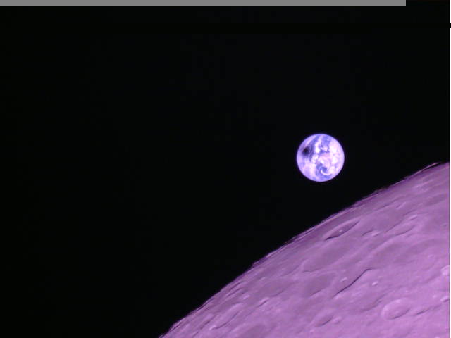
In my previous post, I spoke about the opportunity to take images of the Moon and Earth using the Inory eye camera on DSLWP-B during the first week of June. All the tentative plannings for programming the image taking and downloading the images listed in that post were eventually made final, so the observation runs have been done without any modifications to the schedule.

On June 3, a series of 9 images with 10 minutes of spacing was taken starting at 03:05 UTC. This gives a nice sequence of the Earth hiding behind the Moon and reappearing. One of the images was partially downloaded during the same 2 hour activation of the Amateur payload on June 3. Several of the remaining images were downloaded between June 4 and June 6. On June 7, the station of Reinhard Kuehn DK5LA, which is normally used as the uplink station, wasn’t available, so a single image outside of the Moon series was downloaded using Harbin as uplink station.

This is a report of the images taken and downloaded during this week.

On 2019-03-03, nine images were taken starting at 03:05 with an interval of 10 minutes between each image. These images had IDs 0xC9 to 0xD1 (see this post for more information about image IDs). After the imaging run had finished, between 04:47 and 05:05, coinciding with the payload shut down, image 0xCE shown below was partially downloaded. Only a few chunks of this image were received successfully by the Chinese stations, since Dwingeloo wasn’t online at that time (the Moon was at a low elevation in Europe).

On 2019-06-04 the payload was activated at 07:00. Between 07:09 and 07:45, image 0xCE was completed. After this, image 0xCB was completely downloaded using several transmissions between 07:53 and 08:58. This is probably the best image taken with DSLWP-B so far and the team at Dwingeloo was quite surprised when they downloaded it.

On 2019-06-05 the payload was activated at 07:00. Images 0xCA and 0xCC were downloaded partially. The telemetry server was down during that day, so I have not been able to recover accurate information about the times when the images were downloaded.

On 2019-06-06 the payload was activated at 07:00. Between 07:07 and 07:43, image 0xCD shown below was downloaded completely. Then, between 07:53 and 08:11, image 0xCF shown below was downloaded. After this, between 08:19 and 08:31, image 0xCA shown above was almost completed (note that there is still a small piece of the image missing). Finally, between 08:39 and 9:00, image 0xCC shown above was completed.

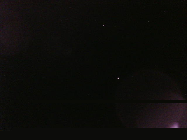
On 2019-06-07 the payload was activated at 08:00. Reinhard was not available, so he couldn’t operate his uplink station. Harbin was used as uplink instead and it was possible to command the download of image 0xD5, which doesn’t belong to the series taken on 2019-06-03, but rather is the image taken as the payload was activated on 2019-06-07. The image is shown below (note that it was only downloaded partially). The main purpose of attempting to download this image was to provide a continuous signal for VLBI, but incidentally it is an interesting image because it contains several visible stars. There is only another image of DSLWP-B showing stars, and these can be used to measure the camera pointing accurately.

From the series of images taken on 2019-06-03, there is still necessary to download 0xC9, 0xD0 and 0xD1, and to complete the missing chunks of 0xCA. The download of these images will probably be attempted on future activations of the Amateur payload.

Wei Mingchuan has colour-corrected the images 0xCB trough 0xCE, and made a very nice animated GIF.

In my last post, I spoke about the images taken by DSLWP-B, the Chinese lunar orbiting Amateur satellite, during the first week of June. One of these images was the picture of stars shown below, taken on 2019-06-07 08:00 UTC.

Although it may seem that this image is not very interesting in comparison with the other awesome images of the Earth and the Moon, the stars that appear in the image can be used as a reference to compute where the camera was aiming. In a previous post, I used an image of stars to compute the field of view of the camera. In this post, I will assess the accuracy in the camera pointing. Currently, there exist only two images of stars taken by DSLWP-B, so it is interesting to try to study these as much as possible.

The DSLWP-B camera is supposed to aim away from the Sun, since in the nominal attitude the solar panel aims directly towards the Sun, and the camera is placed opposite to the solar panel. However, the aiming can be off by a few degrees.

The first step in processing the image is to detect the stars and to match their positions against a database to try to compute the camera orientation, as well as its field of view and any possible distortion introduced in the image. To do so, I have used the web service from Astrometry.net.

The image uploaded to Astrometry.net can be seen here. It has been edited slightly to remove some of the lens flare, since otherwise the service failed to identify the image. We can already see there the stars that the service has identified and some data regarding the image, such as a field of view of 38×28.5 degrees (I estimated 37×28 in my post), and a pointing of right azimuth 16^h 56^m 07.929^s and declination of -19° 29′ 48.998″, between the constellations of Ophiucus and Scorpius.

The position of the Sun, as seen from DSLWP-B in ICRF coordinates is computed in the GMAT script photo_icrf.script. Then a Jupyter notebook with Astropy is used to compute the right ascension and declination of the vector that points away from the Sun. This is the nominal camera pointing, which corresponds to a right ascension of 16^h 58^m 57.1908^s and declination of -22º 41′ 34.728”.

An alternative simpler approach is to use Astropy to compute the position of the Sun as seen from the centre of the Earth. This will not be the same as the position of the Sun as seen by DSLWP-B, since the Earth and DSLWP-B are approximately 400000km away, but it will be close enough. Indeed, in this case, the separation between both positions is 0.1º.

Astrometry.net generates several FITS files with information about the calibration of the image. These can be opened in Astropy. One of the files is a list of positions of the stars identified in the image and their real positions in the sky, both in terms of right ascension and declination and in terms of pixels in the image. It is interesting to study this to see what the error is, and check whether there is any distortion in the image that is not modeled by Astrometry.net. In this case, the RMS error is 0.027º, or 97 arc-seconds, which corresponds to 0.45 pixels.

Another of the files generated by Astrometry.net is a WCS file that allows us to translate between pixel coordinates on the image and right ascension and declination coordinates on the sky using Astropy’s WCS module. This can be used to generate the image below, which has an increased contrast and the viridis color map so that stars are seen more easily, and marks the positions of the brightest stars (as computed by Astropy).

Jupiter can also be seen as the brightest point in the image. Its position was computed in Astropy using the position as seen from Earth. As in the case of the Sun, this is not exactly the same position as seen by DSLWP-B, but the difference is small.

The centre of the image is shown with a white cross, while the nominal camera pointing (the direction away from the Sun) is show with a red cross for comparison. The separation between both is 3º 14′ 51.5131”, which confirms the fact that the camera pointing is usually off by a few degrees.

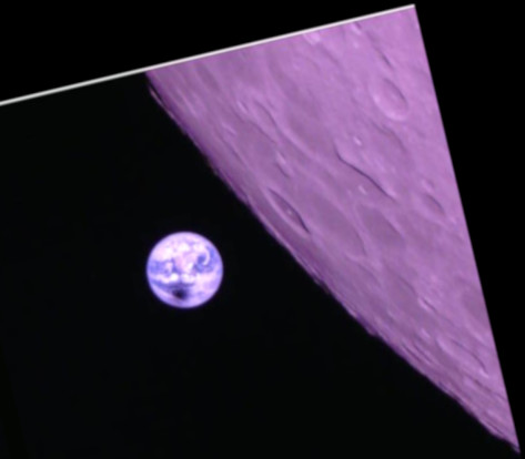
On July 2, there will be a total solar eclipse observable from parts of the Pacific Ocean, Chile and Argentina. This gives the opportunity to image the eclipse with the Inory eye camera on-board DSLWP-B, the Chinese lunar orbiting Amateur satellite. Wei Mingchuan BG2BHC has already started planning for the eclipse observation, and I have run my usual calculations using the 20190618 ephemeris from dlswp_dev.

The main interest in trying to do an imaging session during the eclipse is to photograph the shadow of the Moon on the surface of the Earth. The camera doesn’t have a large resolution, and the Earth looks small in the image, but perhaps it will be possible to distinguish the shadow clearly.

Besides this, it is also interesting to try to get the Moon in the image, as it has been done in other occasions. This not only gives a more interesting picture, but also helps the camera auto-exposure algorithm by providing a large bright object in the field of view. Past attempts to image the Earth alone have all yielded over-exposed images. It turns out that the orbit of DSLWP-B is ideal to image the eclipse, partly by chance and partly because of the nominal satellite attitude.

Recall that the camera of DSLWP-B is always pointing away from the Sun, because the satellite aims its solar panel towards the Sun. Since DSLWP-B orbits the Moon, this means that the Earth will be in the centre of the camera field of view whenever a solar eclipse happens. However, the satellite could be at any point of its orbit. It might happen that the Moon is between the satellite and the Earth, hiding the view, or, more likely, that the Moon is outside of the field of view of the camera.

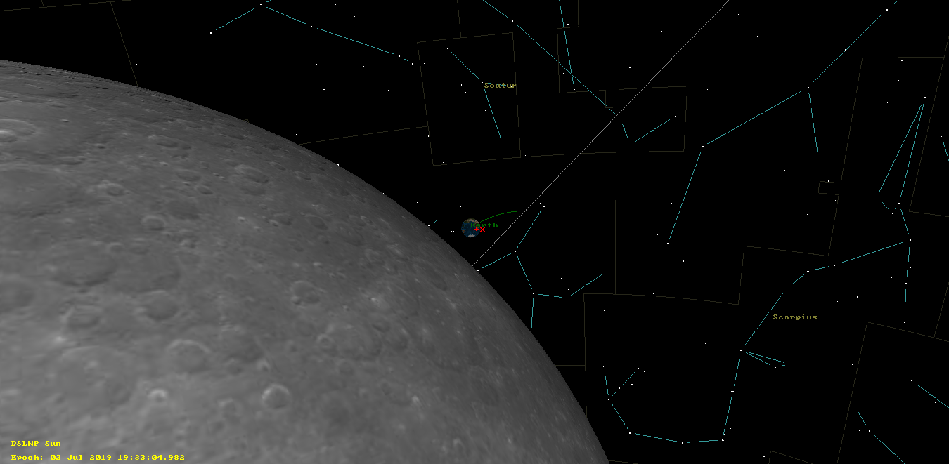
The total eclipse is observable between 18:01 and 20:45 UTC, with the maximum happening at 19:23. The two figures below show the positions of the Moon and Earth within the field of view of the camera. As explained above, the Earth is near the centre of the image during the eclipse. In the bottom figure we see that the Earth is hidden by the Moon until 19:27.

Therefore, it seems that this is an optimal chance to image the eclipse. The Earth will emerge behind the Moon very near to the eclipse maximum. Since DSLWP-B is orbiting at a lower altitude in comparison with other imaging sessions, the Moon will move rather quickly through the camera field of view and disappear in a matter of 10 minutes.

Thus, my recommendation is that instead of taking images every 10 minutes, as it has been done in other occasions, a smaller interval of 2 minutes is used instead. A series of 9 images starting at 19:20 is shown in the plot above as green lines. This gives good coverage of the eclipse and the Earth appearing behind the Moon.

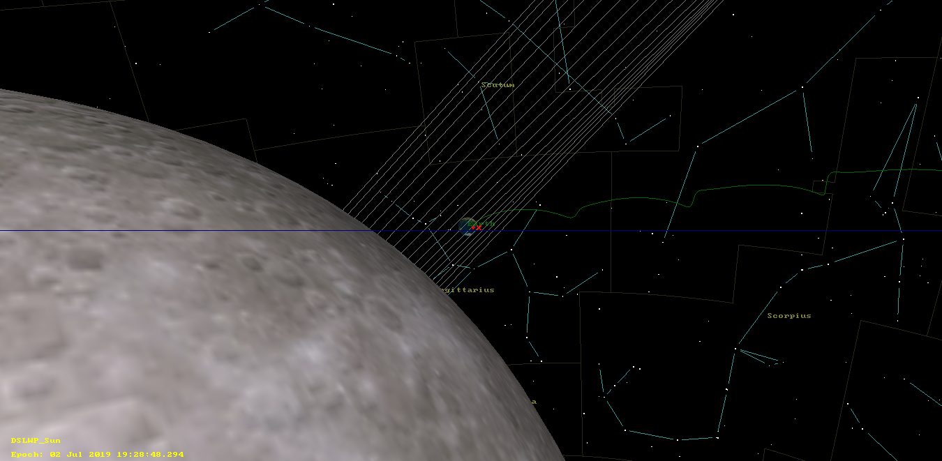
The figure below shows the simulation of the view in GMAT. Note that the field of view of the camera is smaller than what this image shows.

In my last post, I spoke about the possibility of imaging the July 2 solar eclipse using the Inory eye camera on-board DSLWP-B. After discussing the plans for the observations with Wei Mingchuan BG2BHC, we have decided to activate the DSLWP-B Amateur payload during the following intervals:

• 2019-06-30 05:30 to 07:30
• 2019-07-01 05:30 to 07:30
• 2019-07-02 18:00 to 20:00
• 2019-07-03 06:00 to 08:00
• 2019-07-04 06:30 to 08:30
• 2019-07-05 07:30 to 09:30

The camera will be used in 2x zoomed mode, which has a field of view of 14×18.5, degrees. Using the zoomed mode requires careful planning, since part of the Moon needs to appear inside the image, to help the camera auto-exposure algorithm, but the Moon shouldn’t hide the Earth.

The June 30 activation will be used to test the camera, taking images of the Moon in similar positions to those on July 2. The Earth will not be in view of the camera on this day, but these tests will serve to validate camera pointing, exposure, and satellite ephemeris errors.

The following imaging times have been proposed:

• 2019-06-30 05:51:20
• 2019-06-30 05:52:20
• 2019-06-30 05:53:20
• 2019-06-30 06:29:50
• 2019-06-30 06:30:50
• 2019-06-30 06:31:50
• 2019-07-02 18:56:00
• 2019-07-02 18:57:00
• 2019-07-02 18:58:00
• 2019-07-02 19:31:45
• 2019-07-02 19:32:45
• 2019-07-02 19:33:45

The idea for July 2 is to take an image of the Earth and Moon just before the Earth becomes hidden behind the Moon and just after it reappears. Determining these moments accurately is difficult. The Moon will be moving rather fast across the field of view of the camera, since the orbit altitude is rather low. Therefore, the timing of these events is sensitive to the satellite ephemeris and the orbit propagation algorithm. To try to mitigate this effect, we will take a series of three images spaced one minute instead of taking a single image.

On June 30, the same imaging run is mimicked: a series of three images will be taken before the Moon hides the centre of the image (this time the Earth will not be present) and a series of three images will be taken after the centre of the image becomes unblocked again.

The figure below shows the camera view prediction for the June 30 imaging run. The calculations have been done with the 20190630 ephemeris from dslwp_dev.

We note that the second run of three images seems a little early. Wei is doing his calculations with STK and apparently he is getting slightly different orbital predictions compared to my predictions done in GMAT. We haven’t tried to study these differences, but this gives an idea of how sensitive the imaging times are to ephemeris and orbital propagators. Hopefully the series of three images will account for orbital errors. Additionally, after doing the test run on June 30, the results can be compared with the orbital prediction and the imaging times for July 2 can be modified slightly if necessary.

The figure below shows the camera view for the July 2 eclipse imaging run. The 20190630 ephemeris have been used for this plot also. We have the same effect, where the second proposed imaging times seem somewhat early.

Since this time the Earth is also visible in the image, it is convenient to plot the “Earthrise view” plot, which I have used on other occasions. This shows the angular distance between the Earth and the Moon rim, so it can be used to determine if the the Earth is hidden by the Moon (negative distance) or not.

As we can see below, according to my GMAT prediction, the Earth will not be visible in the images around 19:30. It seems these should be taken a few minutes later. However, Wei has obtained different results with STK. In any case, these imaging times can be corrected based on the results obtained on June 30.

The plots in this post have been made in this Jupyter notebook.

As a GNSS engineer at my day job in GMV, it’s not uncommon to find myself looking at spectrums of the GNSS signal bands, either on a spectrum analyzer or on an IQ recording done by an SDR. A few days ago, I spotted something in the L1 band (1575.42MHz) that quickly caught my eye: a pair of strong carriers at +/- 511.5kHz away from the L1 centre frequency. This was visible on some of the recordings that we had done in the last few days, and also live on a spectrum analyzer.

When monitoring the signal on the spectrum analyzer, it disappeared a few hours later, making me suspect that it was transmitted by a satellite rather than a local interferer. Back at home, I did some recordings with STRF to try to identify the satellite using its Doppler.

The Doppler signature of the signal was a perfect match for GPS SVN49, also as USA-203 and GPS IIRM-7. This satellite, launched in 2009, was the first to demonstrate the L5 signal. During in-orbit testing, an anomaly with its navigation signals caused by the L5 filter was discovered. The satellite was never put into operational use, and has been used for varied tests ever since.

After searching information about this satellite, I learned that some researchers from Torino, Italy, had already observed back in 2017 the same kind of signals that I was seeing.

This post is a detailed study of the L1 signal that is currently being broadcast by GPS SVN49. The data used here has been published in Zenodo as “RF recordings of GPS SVN49 broadcasting non-standard codes“.

My recording setup at home is a LimeSDR locked to an external 10MHz reference generated by a DF9NP GPSDO. The antenna is an inexpensive small patch for GPS L1 which has good visibility of the northern sky but limited visibility of the southern sky. The same antenna is used for recording with the LimeSDR and for the GPSDO.

I use STRF to compute and record waterfall data. See this tutorial for more information about STRF. The lime_gnss_iot.grc GNU Radio flowgraph is used to record IQ data at 2Msps to the FIFO /tmp/gnss_fifo, while rffft is run as

rffft -i /tmp/gnss_fifo -f 1575.42e6 -s 2e6 -c 10 -t 100 -F float

to record waterfall data.

The signal of SVN49 is clearly visible in the two spectrums shown below, produced with this Jupyter notebook by reading the data recorded by rffft. The first shows the spectrum before SVN49 is visible in the sky. Three spikes are visible: one is the DC spike and the two others are local interferers.

The second figure shows the spectrum four hours later, after SVN49 has appeared in the sky. Besides the two local interferers that are also present above, spikes at +/- 511.5kHz have appeared. This is the signal broadcast by SVN49 and it is what caught my attention originally, since I had never seen such a signal in the L1 band.

This signal is produced by using a so-called non-standard code. Instead of transmitting a spread spectrum PRN based on a Gold code, the satellite transmits a PRN which consists of alternating zeros and ones. This can be seen as a square wave subcarrier, which produces modulation sidebands at +/- 511.5kHz (half the chipping rate). Instead of spreading the signal power over 2MHz of bandwidth, as the spread spectrum PRNs do, the non-standard code concentrates the signal power in these two spikes.

The figure below shows some waterfall data in rfplot. Approximately between 08:00 and 14:00 UTC the two spikes produced by SVN49 are visible.

Using

rfplot -p 2019-06-25T20\:59\:36 -f 1575.9315e6 -w 10e3 -z 0.01

we can view a waterfall of the upper sideband (the upper spike at 1575.9315MHz) of the modulation. The figure below shows the Doppler curve during one full pass of the satellite. The fainter traces are spectral lines from other GNSS satellites that are using spread spectrum codes.

Doppler data can be extracted from the waterfall above and then processed with rffit to identify the TLE that best matches the Doppler curve (see exercise 6 in this tutorial). The latest TLEs from Space-Track were used.

The TLE for NORAD ID 34661, which corresponds to SVN49, gives the smallest RMS error when fitting the Doppler curve. As shown in the figure, the error is 17Hz. No other satellites produced an error smaller than 100Hz, so the signal is determined to come from SVN49 without any possible doubt.

A more careful look at the signal shows that it is modulated with navigation data. Low rate (5ksps and 10ksps) IQ samples centred on 1575.9315MHz were recorded for later analysis of the modulation. The figure below shows a waterfall of the signal in inspectrum. A 50 baud BPSK modulation is clearly visible. There are other much fainter traces that correspond to spectral lines of other GNSS satellites using spread spectrum modulations. The data modulation is also visible in these.

The bpsk_demod.grc GNU Radio flowgraph is used to demodulate a excerpt of this IQ recording. The flowgraph is shown below. A signal source and VCO blocks are used for coarse Doppler correction, assuming a constant frequency change rate with parameters estimated by eyeball. The BPSK symbols are saved to a file for later processing.

The excerpt processed by this flowgraph is a 3600 second long segment of the usb_modulation_2019-06-25T20:59:41.378538_5ksps.c64, starting at an offset of 49900 seconds. This corresponds to 2019-06-25 10:51:21 UTC. The excerpt is made with

dd if=usb_modulation_iq_2019-06-25T20\:59\:41.378538.c64 of=modulation_excerpt.c64 bs=1000000 count=144 skip=1996

The navigation message is then analyzed in this Jupyter notebook. We refer the reader to that notebook for the detailed analysis. Only a summary is included in this post.

Most of the navigation message data is valid. HOW words with TOWs ranging between 10:52:18 and 11:48:48 have been decoded with successful parity. The remaining data in the TLM and HOW words is valid, but, interestingly, the alert (which indicates a satellite malfunction) and anti-spoofing (which indicates that the P code is encrypted) flags are not set. Subframes 1 through 5 are transmitted in the usual cycle.

The 8 data words (i.e., the words other than the HOW and TOW) for subframes 1 (WN, health and clock), and 2 and 3 (ephemeris) are not valid. A sequence of alternating ones and zeros is transmitted in these words, including over the parity data. This makes the parity of these words invalid. It is interesting that in 2017 the researchers from Torino observed valid ephemeris data.

In contrast, subframes 4 and 5, which contain almanac and other data are valid and contain seemingly good and current almanac data for the complete GPS constellation.

In view of this information, it is interesting to come back to the waterfall of the signal shown above. The data is perfectly visible in the spectrum. Since the contents of subframes 1, 2 and 3 are alternating ones and zeros, these produce a line spectrum. Therefore, each of these subframes is perfectly visible in the waterfall. The contents of subframes 4 and 5 vary a lot depending on which page is transmitted. Therefore, we see different spectral patterns for these subframes, such as a line spectrum indicating periodic data (perhaps anti-spoofing and signal capabilities flags), a carrier indicating constant data (probably all zeros), and a more uniform spectrum indicating more complicated data.

Finally, it is interesting to address the question of when did SVN49 start broadcasting non-standard codes again and if anyone has noticed this before. According to the current IGS MGEX Satellite metadata file, SVN49 broadcasted PRN04 between 2016-02-02 and 2016-09-14 , between 2017-01-06 and 2017-05-13, and between 2017-12-01 and 2018-09-29. I have consulted the U.S. Coast Guard Navigation Center about this non-standard code and they state that SVN49 will transmit the non-standard code whenever it is not in use for other testing purposes.

Thus, shortly after it stopped broadcasting PRN04 in May 2017, the researchers from Torino noticed the presence of the non-standard code. Throughout most of 2018, SVN49 was again broadcasting PRN04, but presumably it was back to the non-standard code on October 2018.

I have searched online for reports of SVN49 transmitting the non-standard code, but I couldn’t find anything besides the article from Torino. Perhaps this is already well known and people do not bother to report it anymore. Still, it is interesting that I haven’t noticed the non-standard code until June 2019. There is perhaps a reason for this.

Currently, SVN49 is visible from Madrid between approximately 06:30 and 14:00 UTC. The orbital period of a GPS satellite is exactly half a sidereal day, so it always repeats the same ground track. However, each day the satellite passes 3 minutes and 56 seconds earlier, so the interval when the satellite is visible from one particular location keeps shifting throughout the year. Therefore, six months ago, SVN49 was visible between 18:30 and 02:00 UTC. Thus, during the summer is when the period where SVN49 is visible from Madrid best matches the normal working hours. So the fact that I have first noticed the non-standard code in June is not completely a mere coincidence.

As described in one of my latest posts, today DSLWP-B has made a test imaging run in preparation for the solar eclipse on July 2. A series of images was taken just before the Moon hid the centre of the camera field of view and just after the Moon left the centre of the image, in approximately the same relative positions as for the July 2 eclipse imaging run.

The activation of the Amateur payload started at 05:30 UTC and the payload was commanded to change the configuration of the camera to use 2x zoom. The satellite was occulted by the Moon at 05:40 UTC, preventing the reception of telemetry until it reappeared at 06:16 UTC. The first series of images was taken automatically between 05:51 and 05:54, with the satellite behind the Moon.

After the satellite reappeared from behind the Moon, telemetry confirmed that three images, with IDs 0xD9, 0xDA and 0xDB had been taken. Between 06:29 and and 06:32, the satellite took the second series of images. Telemetry confirmed that these images were taken correctly with IDs 0xDC, 0xDD and 0xDE.

The priority was to use the rest of the activation to download images 0xDA and 0xDD, taken respectively at 05:52:40 and 06:31:10 UTC (when reading the times given in the planning post, note that the times listed there are the moments when the command is sent to the payload by the satellite, but the payload needs about 20 additional seconds to take the image). However, there were difficulties in commanding the payload, so half an hour was lost trying to command the satellite and only image 0xDA could be downloaded before the payload went off at 07:30 UTC.

Image 0xDA was downloaded without errors in a single transmission. It is shown below.

As we see, the exposure of the image is correct, so this image validates that the camera configuration can be used for the eclipse imaging run. Additionally, the image can be used to evaluate camera pointing and ephemeris errors.

As computed in this Jupyter notebook, the separation between the Moon rim and the centre of the field of view in the image shown above is 6.47 degrees. Using the camera calculations Jupyter notebook that I have shown in previous posts, we see that, according to the 20190630 ephemeris from dslwp_dev and my GMAT calculations, the angular distance between the Moon rim and the centre of the image at 05:52:40 UTC should be 3.25 degrees, assuming that the camera points perfectly away from the Sun.

The rate at which the Moon rim moves through the field of view is approximately 0.029 degrees per second. Thus, if the camera was pointing perfectly away from the Sun, this would indicate that DSLWP-B is 110 seconds earlier in its orbit that what predicted by the ephemeris, so that events concerning the relative position of the satellite and the Moon happen 110 seconds later than predicted.

However, one should take these calculations with a grain of salt. In my astrometry post, I showed that the camera was pointing 3.25 degrees off-axis. Therefore, it is convenient to assume an error of +/-3.25 degrees in the angle measurement done with the image. In units of time, this is +/-111 seconds.

So the data seems to suggest that DSLWP-B is one or two minutes earlier in its orbit and that the imaging times should be compensated by making them one or two minutes later, but there is not enough statistical evidence to support this argument. It will be very interesting to see image 0xDD, which will be downloaded tomorrow. The analysis of this image will give additional data.

In any case, so far it seems that orbit and pointing errors are within the tolerance given by the series of three images, which are taken at -1, 0, and +1 minutes offset from the nominal imaging time computed by Wei.

Yesterday I did an analysis of the image taken and downloaded during the test run for the imaging of the solar eclipse shadow on the Earth with DSLWP-B on July 2. Only one of the six images taken to validate the camera exposure and pointing and orbit errors was downloaded yesterday. The window to download the remaining images was during today’s activation of the Amateur payload between 05:30 and 07:30 UTC.

Three images were downloaded today, with a few missing chunks. Moreover, Wei Mingchuan BG2BHC has sent me better ephemeris, which give a more accurate prediction of the orbit both on the June 30 test run and on the eclipse imaging run on July 2. This post is an analysis of the images downloaded today.

Images 0xDD, 0xDE and 0xDB from the series of six test run images (0xDA – 0xDE) were downloaded from DSLWP-B, using the groundstation at Dwingeloo. These are shown below. As it can be seen in the captions, most of the time the satellite was kept transmitting an image, so an efficient use was made of the two hour activation window.

In parallel, the GMSK to JT4G repeater onboard DSLWP-B was used to make a QSO between BY2HIT, the Harbin Institute of Technology Amateur radio club, and Reinhard Kuehn DK5LA. This is the first ever Amateur radio QSO made through a lunar orbiting repeater. It was reported by Wei in the tweet shown below.

Using the GMSK to JT4G repeater is not easy, in terms of the signal power needed for the uplink. There were plans to make a QSO between BY2HIT and Reinhard since many months ago, but previous attempts didn’t work out. My congratulations to the people at both sides of the QSO, who have achieved it a month before DSLWP-B crashes against the lunar surface.

The GMSK to JT4G repeater works by sending commands to the satellite which embed a 13 character message, using the same frequency and a similar protocol to the one used to command the camera and other satellite functions. The precise definition of this mode is a 7.8125 baud FSK modulation with a shift of 394.53125Hz. Each FSK tone is “spread” with a 250 baud GMSK 32 bit syncword. The CCSDS 32 bit syncword is used to mark the beginning of a packet, and a Reed-Solomon (64,32) code is used for FEC, together with CCSDS scrambling. Such a message takes a bit longer than one minute to transmit. The uplink is in the 2m Amateur satellite band.

The repeater downlink is the usual JT4G downlink of DSLWP-B in the 70cm Amateur satellite band. The 13 character messages sent in the uplink command replace the usual JT4G telemetry, being repeated as a free-form JT4G message. In the case of this QSO, the B1 radio at 436.400MHz was used. This radio was also used to transmit the images using GMSK SSDV.

I have updated my Jupyter notebook to measure the angle between the centre of the image and the rim of the Moon in each of the images downloaded today. Angles of -1.33º, 1.31º and 4.70º have been obtained for images 0xDD, 0xDE and 0xDA respectively.

Since I suspected that the usual ECEF cartesian ephemeris that Wei computes with STK could be giving some problems, he has been kind enough to share Moon centred ICRF Keplerian ephemeris. These are shown below in GMAT. The only difference from the ephemeris that Wei sent me is that Wei uses a mean anomaly of 164.619 degrees, whereas GMAT needs the true anomaly. The true anomaly below has been computed from this mean anomaly and the eccentricity.

DSLWP_B.DateFormat = UTCGregorian;
DSLWP_B.Epoch = '28 Jun 2019 03:00:00.000';
DSLWP_B.CoordinateSystem = LunaICRF;
DSLWP_B.DisplayStateType = Keplerian;
DSLWP_B.SMA = 8704.163;
DSLWP_B.ECC = 0.690187;
DSLWP_B.INC = 44.672;
DSLWP_B.RAAN = 71.711;
DSLWP_B.AOP = 68.006;
DSLWP_B.TA = 176.09042928330206;

I have redone the graphs in this post using these ephemeris. The results are shown below.

It is interesting to compare these figures with the figures computed with the ECEF ephemeris. The times when the Moon passes through the centre of the image have changed slightly, and now match much better the times that Wei proposed for taking the images. Therefore, I think that using the ICRF ephemeris in GMAT we get results that are very similar to what Wei is getting in STK.

Using this data, we can compute the difference in the separation of the Moon rim from the centre of the image as measured in the images and as predicted by the ephemeris. This is done in the camera view Jupyter notebook. We obtain values of 3.53º and 3.54º for images 0xDB and 0xDC, which were taken as the Moon hid the centre of the image, and -3.34º and -3.19º for images 0xDD and 0xDE, which were taken as the Moon moved again out of the centre of the image.

Note the different signs in these values. As the Moon was moving towards the centre of the image, we have positive differences, meaning that the Moon was further from the centre of the image than what predicted by the ephemeris. As the Moon was moving away from the centre of the image, the Moon was closer to the centre of the image than what predicted.

These results are consistent with the idea I introduced in the previous post that the satellite is somewhat earlier on its orbit than what is predicted by the ephemeris. On the other hand, the difference between the ephemeris prediction and the images could be caused by a pointing error. However, assuming that the satellite didn’t change its attitude noticeably throughout the test run, a pointing error would contribute with the same sign to all the images.

Taking into account the speed at which the Moon moves through the field of view, as predicted by the ephemeris, and assuming no pointing error, we get a temporal error in the along-track component of the orbit of -120, -118, -81 and -77 seconds on each of the images.

Even though we have assumed that there can be a pointing error of up to 3.25º, which represents a temporal error between 78 and 113 seconds, the data seems to suggest that most of the discrepancy between the images and the ephemeris prediction is caused by an along-track error in the orbit. A pointing error of around 1.4º towards the left of the image could explain the relatively large difference of along-track errors seen when the Moon moves into the image (around -120 seconds) and when the Moon moves away from the image (around -80 seconds). In this case, the real along-track error would be on the order of -100 seconds.

Even though I reckon that these images are not a very precise tool for measuring the orbit, my guess is that DSLWP-B is between one and two minutes earlier on its orbit than what predicted by the ephemeris. This is not much of a problem for tomorrow’s eclipse imaging, because several images will be taken and there is some margin for error. The only risk is that in some of the three images taken as the satellite reappears from behind the Moon, the Earth might still be hidden. Additionally, Wei tells us that it is not so easy to change the programmed imaging times at this point, so let’s hope for the best tomorrow.

Probably you’ve already seen the amazing images of the July 2 solar eclipse taken by DSLWP-B. These have have been shared in Twitter by the Harbin Institute of Technology Amateur Radio club BY2HIT, Tammo Jan Dijkema from the Dwingeloo radiotelescope in the Netherlands, and others.

I have devoted the last few posts to the planning of the imaging times for the eclipse test run and the validation of the test run done on June 30. This post is a detailed account of the results of the eclipse imaging. Between July 3 and 5, five of the six eclipse images taken on July 2 were downloaded, as well as some other images taken later. Here I give a summary of the downloads during these days and compare the images to the predictions I made.

Log of activities between July 3 and 5

The six images taken during the eclipse run had IDs between 0xE1 and 0xE6 (see this post for more information about image IDs). The times at which the images were taken are listed in this post, but keep in mind that these are the times at which the imaging command is sent to the Amateur payload on board DSLWP-B. The payload takes the image approximately 20 seconds after it receives the command.

On July 3, the Amateur payload was activated between 06:00 and 08:00 UTC. The downloading activities were planned and executed very efficiently by Wei Mingchuan BG2BHC, who coordinated the activities, Reinhard Kuehn DK5LA, who operated the uplink station in Germany, and the people operating the Dwingeloo 25m radiotelescope in the Netherlands, which was the main downlink station. Secondary downlink stations at Harbin and Shahe, in China, and Wakayama, in Japan, were used some of the days.

A total of four complete images from the eclipse could be downloaded on July 3. All the DSLWP-B team as well as people following on Twitter were truly impressed with the quality of the images. I was quite relieved when seeing that the Earth was well separated from the Moon in many of the images. My main concern when planning the observations was that an inappropriate imaging time would cause the Earth to be hidden behind the Moon.

The four images downloaded on July 3 are shown below.

On July 4, the payload was active between 06:30 and 08:30 UTC. First, a few minutes were spent to download the first chunk of image 0xE6, which was missing in the July 3 download.

There is a well known bug with the DSLWP-B SSDV system used to transmit the images that causes the image transmission to start by the second chunk instead of the first one whenever a complete image transmission is requested, so the first chunk is skipped. In many images this first chunk is completely black so its download is not needed, but in others it has to be downloaded manually later on.

The complete image 0xE6 is shown below.

Next, image 0xE4 was downloaded. This was the first of the three images taken as DSLWP-B came out of the occultation. In this image, the Earth is hidden behind the Moon. DSLWP-B is moving towards the lower right corner of the image, so some seconds after this image was taken the Earth would have become visible. Compare with image 0xE5 shown above, which was taken one minute later.

After downloading this image, the settings of the camera were changed to take an image of a field of stars. This involves changing the camera exposure for reduced lighting conditions. The command to take the image was sent by Reinhard around 07:56, so the image was taken approximately at 07:57, since the commands take one minute to be sent.

The download of the image was commanded, but instead of getting an image of stars we got a purple lens flare as we have seen in other occasions. The reason for this is that the Earth was still in the field of view of the camera, overexposing the image. Therefore, the download of the image was commanded to stop, as this kind of image is not very interesting and it is better to devote the time in which the payload is active to other activities.

After stopping the download of image 0xE9, the download of image 0xDC was started. This is one of the images which were taken during the June 30 test run, and which hadn’t been downloaded yet. However, the payload shut off a few minutes after the download started, so only the top part of the image could be downloaded, as shown below.

On July 5, the payload was active between 07:30 and 09:30 UTC. The first task during the activation was to download again image 0xDC. This was completely downloaded, and is shown in the figure below.

This day, a team of the Chinese NCLE delegation was visiting the Astron premises, where the 25m radiotelescope is housed, so they were taken on a tour of the facilities and given a live demo of the DSLWP-B capabilities at the radiotelescope. The demo consisted in taking and downloading some pictures of the lunar surface.

The plan was to download image 0xE1 after 0xDC. This image was the first of the July 2 eclipse images, and the only one among the six images which hadn’t been downloaded yet. Then, pictures of the Moon surface would be taken manually at 08:25 and 08:29, the satellite would hide behind the Moon between 08:31 and 08:59, and the lunar surface images would be downloaded after the satellite reappeared.

However, image 0xE1 could not be downloaded due to timing constraints, and the command for taking the image at 08:29 wasn’t successful. The command sent at 08:25 did indeed work, and this image could be downloaded almost completely before the payload switched off.

It is quite interesting that this image doesn’t have the peculiar purple hue that is present in almost all the other DSLWP-B images. Indeed, only a few other images taken during the first three months of the mission look yellowish like this one. It was assumed that at some point the yellow channel of the camera sensor might have failed.

However, it seems that the hue has something to do with the exposure settings of the camera. This image was taken with the shortest exposure possible, since the Moon surface would completely fill the image. Most other images don’t use the shortest exposure setting, since the Moon only fills part of the image.

Analysis of the eclipse images

Here I study the July 2 eclipse images obtained by DSLWP-B to compare the positions of the Earth and Moon in the images with the predictions I obtained using GMAT and my camera view Python scripts. The Moon centred ICRF ephemeris given in this post are used here.

In the analysis of the June 30 test run images, I measured the angular distance between the rim of the Moon and the centre of the image. This measurement has the problem that it is sensitive to camera pointing errors. In the eclipse images it is better to measure the separation between the rims of the Earth and the Moon, as this quantity is insensitive to camera pointing errors. For simplicity, only images 0xE2, 0xE5 and 0xE6, in which the Earth is completely visible, are used in the study.

This Jupyter notebook is used to measure the distance between the borders of the Earth and the Moon in pixels. This is then converted to an angular distance in degrees by using the resolution of 107 arcseconds per pixel that I obtained with the astrometry study of the camera (the resolution obtained there was 214 arcseconds per pixel, but here the camera is used with a 2x zoom factor).

The angular distances obtained from the images are then compared to the values obtained from the orbital simulation using the camera view Jupyter notebook. Differences of 0.47, -0.69 and -0.56 degrees are obtained respectively for each of the images.

These differences can be transformed into a temporal difference by dividing by the derivative of the angular distance between the Earth and Moon rims. Doing this, we obtain values of -13.2, -12.9 and -10.8 seconds. Assuming that the ephemeris describe the orbit exactly, this would mean that the images have been taken between 11 and 13 seconds before their nominal times. An alternative explanation is that the images have been taken at their nominal times but DSLWP-B is some 12 seconds earlier in its orbit than what described by the ephemeris.

Since the 20 seconds between the time the command is sent to the payload and the moment that the image is taken is just and approximation, it is not so easy to tell which of these effects is causing the temporal difference of around 12 seconds. Additionally, sometimes the DSLWP-B on board clock is a few seconds off. This would give a third possible explanation.

The only additional data we have to constrain DSLWP-B’s orbit are Scott Tilley VE7TIL’s radio occultation measurements of the S-band beacon done on July 1. After I analyzed the June 30 test run images, Scott was kind enough to observe a radio occultation on short notice.

When DSLWP-B hides behind the Moon, its radio signal disappears. By measuring the exact moments at which the radio signal disappears and the moment at which it reappears back, it is possible to get constraints on the orbital parameters. One of the parameters best constrained by this measurement is the mean anomaly, since an error in mean anomaly will put the satellite somewhat sooner or later in its orbit, shifting both occultation timestamps by the same amount in comparison to the prediction.

Scott measured the start of the occultation to be at 2019-07-01 22:29:02UTC, and the end of the occultation to be at 2019-07-01 23:05:26 UTC. According to my GMAT calculations, which take into account the finite propagation speed of light, the occultation observed by Scott should have started at 22:29:00 and ended at 23:05:15. Therefore, we have an error of -2 seconds in the beginning of the occultation and -11 seconds in the end of the occultation (meaning that the satellite is slightly earlier on its orbit than predicted). This can serve to explain part (or even all) of the temporal difference observed between the images and the prediction.

Another interesting thing to study in the eclipse images is the camera pointing error. This was the main source of confusion when I studied the test run images, since there it was difficult to distinguish a pointing error from an orbit error. In the eclipse images, however, it is very easy to study the pointing error.

Recall that, nominally, the DSLWP-B inory eye camera always points away from the Sun, since it is placed on the opposite side of the solar panel, which is kept pointing towards the Sun. The centre of the eclipse shadow that is seen on the Earth’s surface is located in the line joining the centres of the Moon and the Sun. If the satellite was also placed on this line, then the away-from-Sun vector of the camera would point to the eclipse shadow. Since the satellite is not so far away from the Moon, we can do an approximation and take the eclipse shadow as the away-from-Sun vector. This means that, if the camera pointing was perfect, the eclipse shadow would be centred in the image.

I have measured by hand the location of the eclipse shadow in each of the four eclipse images where it is visible. These locations are shown in the figure below together with one of the eclipse images for reference. I have also included the away-from-Sun vector that I measured in the astrometry image. That image was taken with a 1x zoom factor, while the eclipse images have been taken with a 2x zoom factor, so the position of the away-from-Sun vector, marked as an orange cross, has been corrected for the difference in zoom factor.

The figure above shows that the pointing error direction and magnitude is very consistent, even between the eclipse images and the astrometry image, which was taken almost a month before the eclipse. The pointing error is approximately 3.3 degrees, roughly towards the lower left corner of the field of view (the crosses should appear in the centre of the image).

This suggests that the most of the pointing error is not caused by an error in the ADCS system DSLWP-B, but rather by the fact that the camera is probably not installed perfectly aligned with the satellite body axes.

Now that the DSLWP-B eclipse images have become widespread, appearing even in some newspapers, I have taken the time to identify the features of the lunar surface that can be seen in two of the images. As with any Earth and Moon pictures of DSLWP-B, the part of the Moon that can be seen in these images belongs to the far side, with longitudes of approximately 100º E and 100º W (the division between the near side and the far side happens at 90º E and 90º W, and 0º is the middle of the near side).

I have compared the images with a simulation of the camera view done in GMAT. Using this simulation as a reference and these lunar surface maps as well as Google Moon, I have labelled the features that are visible in the images. The 4K lunar surface map from Celestia Motherlode has been used in GMAT, instead of the default, lower resolution map.

Occultation entry

The figure below shows the GMAT camera view simulation for one of the images taken as DSLWP-B was hiding behind the Moon. The field of view in this figure is much larger than the field of view of the DSLWP-B Inory eye camera. The up direction is the normal to DSLWP-B’s orbit around the Sun (defined as the plane containing the position and velocity vectors with DLSWP-B with respect to the Sun). Therefore, it points approximately towards the north pole. DSWLP-B is moving towards the upper right corner of this image.

The figure belows shows the ground track view. The satellite has crossed the near side and is now starting to orbit over the far side, soon becoming hidden behind the Moon.

Image 0xE2, taken on 2019-07-02 18:57:20 is shown below. The image has been rotated to match the orientation of the GMAT camera view simulation.

The craters that are visible in this image are labeled in the figure below. These belong to the Mare Australe region, and several well known craters such as Jenner and Lamb can be seen.

Tammo Jan Dijkema has done a similar exercise with image 0xE3, which was taken a minute after the image shown above. DSLWP-B has moved towards the upper right corner of the image, so that a larger portion of the lunar surface is visible.

Occultation exit

The figure below shows the GMAT camera view simulation corresponding to image 0xE5, which was taken shortly after DSLWP-B exited the occultation, so that the Earth was visible again.

Below we see the ground track corresponding to this image. The satellite has crossed the far side of the Moon in a south to north direction and soon will cross over to the near side.

The figure below is image 0xE5, which was taken on 2019-07-02 19:33:05. It has been rotated to match the orientation of the GMAT simulation.

The craters are labelled in the figure below. Important craters in the Coulomb-Sarton basin such as Stefan and Bragg are visible. An image of this region with the craters labelled can be seen here.

During this week, the Amateur payload of DSLWP-B has been active on the following slots:

• 2019-07-09 12:30 to 14:30 UTC
• 2019-07-10 13:50 to 15:50 UTC
• 2019-07-12 02:00 to 04:00 UTC
• 2019-07-12 16:30 to 18:30 UTC

In these activations, the last remaining image of the eclipse was downloaded. Also, images of the lunar surface as well as stars have been taken and downloaded. This post is a summary of the activities made with DSLWP-B over the week.

2019-07-09

On July 9, image 0xE1 was downloaded. This was the first image in the eclipse imaging run and the only one which hadn’t been downloaded yet. It is shown in the figure below.

After that, some missing chunks of image 0xEA were downloaded. This image was taken and downloaded on July 5, as part of a demo to the Chinese NCLE delegation during their visit to Astron.

To identify to what part of the Moon surface this image corresponds to, I have used a GMAT script with the Moon centred ICRF ephemeris from June 28, in the same manner as in my previous post. This GMAT script shows a simulation of the camera field of view. The two figures below show the field of view and the ground track corresponding to image 0xEA.

This has enabled me to identify the lunar features that can be seen in the image, even though the contrast is low. The main feature is the Sklodowska crater, which can be identified by its characteristic two small craters on opposite sides of the rim of the main crater. These small craters are approximately 10km in diameter, so it gives an idea of the size of the features that can be resolved by the Inory eye camera.

In the image above, which shows the simulated camera image (but with a much wider field of view), Tsiolkovskiy crater is visible as the characteristic dark crater on the right, and the Mare Australe can be found near the bottom. The Sklodowska crater is near the centre of the image.

After the download of image 0xEA, a new image of the lunar surface was taken at 14:18 UTC. The download of the image was started shortly after this, but the payload shut down before most of the image could be transmitted. The partial image is shown in the figure below.

2019-07-10

On July 10, an image of stars was taken approximately at 14:01, and then downloaded. The image is shown below, but most of the stars are too faint to be seen easily without increasing the contrast of the image.

The team at Dwingeloo performed the following image identification with Astrometry.net. The camera looks into the constellation of Sagitarius, as expected given the locations of the Earth and the Sun at this time of the year (the Inory eye camera always points away from the Sun). The brightest object in the image is Saturn.

After downloading image 0xF1 shown above, another image of stars was taken and downloaded. This image is very similar to the one above, since they were taken only 17 minutes apart. The only difference is in a small rotation of the camera, probably caused by a small attitude change of DSLWP-B.

I have used Astrometry.net to identify the image above (or rather, an enhanced contrast version, to help the star identification algorithm).

After the two images of stars were downloaded, image 0xEE, which was taken on July 9 at 14:17 UTC was downloaded. This image shows a part of the lunar surface. It was first identified as being the Goddard crater by Achim Vollhardt DH2VA on Twitter. The bright small crater is Goddard A, which is 12km in diameter. It is interesting to compare it to the small 10km craters in the Sklodowska crater image. The resolution of this Goddard crater image is approximately 200m per pixel, so not bad at all.

The figures below show the GMAT simulation for this image. The Goddard crater is clearly visible near the centre of the image.

2019-07-12

On July 12, the payload was active in two slots. In the first slot, the Moon wasn’t visible from Europe, so only some telemetry was received in China and the USA. This slot was used to take a series of five images at the following times: 02:00, 02:59, 03:00, 03:01, 03:02. These images have IDs from 0xF3 to 0xF7.

During the second slot, the Moon was visible from Europe, so Dwingeloo acted as the main downlink station as usual. First, a few missing chunks from the Goddard crater image were downloaded.

Then, image 0xF8, which was taken at the payload power on of this slot was downloaded. This image shows a field of stars very similar to the two images shown above. Its Astrometry.net identification can be found here.

After downloading this image, image 0xF7, which was taken during the first slot was downloaded. This is an image of the lunar surface.

In this image, Mare Anguis is visible as some darker patches at the left hand side of the image. The remaining part of the image shows the area northeast of Mare Anguis. The figures below show the GMAT simulation corresponding to this image.

Mare Anguis is shown near the bottom of this image. It seems to be rather far from the centre of the image. The discrepancy might be explained by the fact that the satellite was passing the periapsis, where its speed is highest and distance to the lunar surface is lowest, so a small error in the ephemeris would cause a large difference in the imaged area.

You may have already heard that the Galileo EU satellite navigation constellation is out of service since last Thursday July 11th. Currently the Galileo constellation status page shows that the status of most Galileo satellites is not usable because of a service outage. The satellites not affected by this outage are E20, which was made unavailable on 2014-05-27, and E14 and E18, the Galileo eccentric satellites, which failed to achieve the circular nominal orbit and are only used for testing purposes.

The European GNSS Agency has given very little information regarding the causes of the problem. The available information boils down to NAGU 2019026, posted on 2019-07-13 20:15, which states that starting from 2019-07-12 01:50 the Galileo signals should not be used.

This has originated many rumours and confusion about the problem. It seems that the major cause was a failure in the Precise Timing Facility, which is in charge of the generation of a realization of the GST, the timescale used by Galileo. This has affected the OSPF, which is the service that generates the orbit and clock products (ephemeris) for the satellites. Thus, since Thursday, no new ephemeris are being computed and uploaded to the satellites.

Taking rumours aside, in this post I will look at some facts about the outage which can be learned by analizing the Galileo signal. Other people have published similar studies, such as the NAVSAS group from University of Torino.

This study is based on an observation done between 2019-07-15 22:00 and 2019-07-16 05:30 UTC approximately. I recorded the Galileo E1 band using a LimeSDR, a sampling rate of 4Msps and a resolution of 1 bit. The E1B signal was later processed with GNSS-SDR to obtain the ephemeris and almanac data. The GNSS station I have at home is rather modest, with a small patch antenna having a good part of the southern sky blocked, and a long run of coaxial cable to the LimeSDR. Therefore, the performance is far from ideal, but it is still possible to track a few of the satellites in view with GNSS-SDR.

The output of the Galileo navigation and almanac data produced with GNSS-SDR is stored in this gist as XML files.

As far as I have been able to check, all the aspects of the modulation of the Galileo signals are working correctly. The navigation message also contains the correct week number and time of week, since these are generated on-board the satellite.

However, a look at the gal_ephemeris.xml file shows the ephemeris are stuck in the past. All the satellites are broadcasting an ephemeris set with an \(\mathrm{IOD}_{\mathrm{nav}}\) of 958 and a \(t_{0e}\) and \(t_{0c}\) of 424200, which corresponds to Thursday 21:50. This is the last valid batch of ephemeris that was transmitted on Thursday 11th, right after \(\mathrm{IOD}_{\mathrm{nav}}\) 831, which corresponded to 18:50. Since that date, no new ephemeris have been transmitted. The satellites keep transmitting \(\mathrm{IOD}_{\mathrm{nav}}\) 958 continuously.

It is also possible to check this in the Broadcast Ephemeris products of the MGEX, such as brdm1920.19p.Z, or in the MGEX data for individual stations, such as the data for the VILL station in ESAC.

The ephemeris sets are transmitted only with a time of week parameter. There is no week number associated to them, so a receiver will compute the day corresponding to the ephemeris batch by taking the day with such time of week that is nearest to the current date. This means that when the ephemeris are more than 3.5 days old, they will be assigned to an incorrect day by the receivers. In the case of this outage, this has happened at 2019-07-15 09:50. After this moment, the broadcast ephemeris are no longer assigned to last Thursday 11th, but rather to next Thursday July 18th.

Ephemeris older than a few hours (4 hours is usually taken as a limit) should not be used for navigation, since the orbital errors start increasing above the metric level. This is the reason why the outage was declared at 2019-07-12 01:50 UTC, when \(\mathrm{IOD}_{\mathrm{nav}}\) 958 was 4 hours old. However, the precision of the ephemeris is still on the order of hundreds of metres or a few km even after a few days of age (see this post for a related study with TLEs for LEO satellites, rather than GNSS ephemeris).

The problem is that misidentifying the day associated to an ephemeris batch will cause huge orbit errors, because the time to propagate the ephemeris is computed incorrectly. Therefore, since 2019-07-15 09:50 we are seeing reports of receivers giving absurd positions for Galileo satellites, such as negative elevations.

In abnormal situations such as this one, it is also interesting to look at the navigation data validity and signal health status bits of the navigation message. The meaning of these is not so straightforward, so it is worth to take a look at page 52 of the Galileo OS SIS ICD.

The INAV pages transmitted in the E1B and E5b signals have independent data validity and health bits for each of these two signals. The meaning of the data validity and health is different. The data validity refers to whether the navigation message is valid or not, and the health refers to the signal and modulation. A signal can be transmitted correctly by the satellite and a receiver may be able to track it normally, but the navigation message modulated on that signal may be erroneous or non-nexistent.

The value of the data validity status bit can be either 0, which indicates “navigation data valid”; or 1, which indicates “working without guarantee”. This “working without guarantee” term is a somewhat peculiar way of saying “not OK”, but I guess that the rationale behind it is as follows: If the navigation message is completely screwed up, then you are not even going to be able to get to this field (because of CRC failure, word 5 not being transmitted, or whatever). However, if you are able to get to this field and see a 1, it means that the navigation message is not so badly corrupted, but you still shouldn’t trust it.

The signal health status field has two bits, so it supports four different values: 0 for “signal OK”, 1 for “signal out of service”, 2 for “signal will be out of service”, and 3 for “signal component currently in test”. Keep in mind that these values refer not only to the signal being currently tracked, since an INAV page has fields for both E1B and E5b and the almanac entries also include the health status of each of the satellites in the constellation. Therefore, it is perfectly normal to see a “signal out of service” somewhere, probably referring to a signal other than the one currently being tracked (which is most likely not out of service).

The gal_ephemeris.xml file shows that the E1B and E5b health status is 0 (OK) for all the satellites tracked in the recording: E01, E03, E04, E05, E09, E11, E19, E21, E24, E25, E31, E33 and E36. This makes sense, because the signal modulation has not been affected by the outage.

The behaviour of the data validity status is more interesting. Satellites E01, E03, E04, E09, E24, E25 and E36 show a value of 0 (OK) for both E1B and E5b, while satellites E05, E11, E19, E21, E31 and E33 show a value of 1 (not OK) for both E1B and E5B. Of course, the correct data validity status in this outage situation is 1.

The reason why only half of the satellites are showing a data validity status of 1 is unknown. I have heard rumour that depending on the on-board software, some satellites are able to detect that the ephemeris are too old and set the data validity to 1 automatically, while others need to be commanded by a groundstation. This still leaves open the question of why haven’t all the satellites being commanded to transmit a data validity status of 1.

The report by the NAVSAS group includes similar results, showing a more extensive list of what satellites have the data validity status bit set to 1.

Finally, it is interesting to take a look at the almanacs in the gal_almanac.xml file. This file contains almanac entries for E01, E02, E03, E04, E05, E07, E08, E09, E11, E12, E13, E15, E19, E21, E24, E25, E26, E27, E30, E31, E33 and E36, which were all the active satellites before the outage. The TOW and WN for each of the almanac entries in this file corresponds to 2019-07-11 00:50. The health status for all the satellites is 0 (OK), except for E02 and E26, which have a status of 2 (will be out of service) for the E1B signal.

In my previous post I wrote about the outage of the Galileo EU satellite navigation constellation that started on 2019-07-12 01:50 GST. For several days, all the Galileo satellites kept transmitting the same batch of ephemeris, which corresponded to 2019-07-11 21:50 GST, rather than sending updated batches of ephemeris.

This situation continued until around 2019-07-16 19:00, when several people reported that they were receiving updated ephemeris from some Galileo satellites. These ephemeris could be used for navigation correctly. The NAVSAS group from University of Torino has published a post where they show, for each satellite, when the updated ephemeris were first received by their equipment in Torino, Italy.

The restoration of the system was publicly announced with NAGU 2019027, published on 2019-07-18 08:20. This NAGU stated that starting from 2019-07-17 20:52 the service was restored, but users might experience some instability.

It is interesting to look at the MGEX broadcast ephemeris to see what happened between 2019-07-16 19:00, when users started to see updated ephemeris, and 2019-07-18, when the system was considered to be fully restored. In this post, I do a detailed analysis of the broadcast ephemeris.

I will use the IGS BRDC files, which are multiconstellation navigation RINEX files obtained by merging navigation RINEX files generated by receivers throughout the world. The advantage of using merged RINEX files rather than a single station as the NAVSAS group did is having a global view of the whole constellation. A single station can only monitor the satellites that it has in view.

The tool I have used to process navigation RINEX files is georinex. This is a Python library that allows one to load observation or navigation RINEX files as an xarray Dataset. This makes it easy to process all the information in the file and represent it graphically.

In doing this, I have found two difficulties. The first is that when georinex loads a navigation RINEX file, it ignores entries which have a duplicated SVN and timestamp. This is done because, without filtering out duplicates, the xarray Dataset that georinex generates would have duplicated coordinate labels, and many features of xarray do not work well with these duplicated labels. Often, RINEX entries with duplicated SVN and timestamp will have exactly the same data, so nothing is lost by filtering out the duplicates.

However, in the case of Galileo, the different I/NAV and F/NAV pages give rise to duplicated entries which do not have the same data. As shown in page A25 of the RINEX 3.03 format description, these are distinguished by the value of the data sources field. This field has the following possible values:

• 0x201, which means that the data comes from E1B I/NAV, the clock data and SISA refer to the E5b,E1 signal pair and only the DVS and HS bits for E5b and E1 are valid.
• 0x102, which means that the data comes from E5aI F/NAV and the clock data and SISA refer to the E5a,E1 signal pair and only the DVS and HS bits for E5b are valid.
• 0x204, which means that the data comes from E5bI I/NAV, the clock data and SISA refer to the E5b,E1 signal pair and only the DVS and HS bits for E5b and E1 are valid.
• 0x205, which means that the data is merged from E5bI I/NAV and E1B I/NAV, the clock data and SISA refer to the E5b,E1 signal pair and only the DVS and HS bits for E5b and E1 are valid.

It is expected that entries with data source values of 0x201, 0x204 and 0x205 will contain the same data, since the I/NAV pages in E5bI and E1B should transmit exactly the same information. However, if one is interested in looking at the DVS and HS bits of all the signals, it is necessary to collect entries with a data source value of 0x102 and at least one of 0x201, 0x204, 0x205.

Since there is no way to collect all this information with georinex, I have made a modification that doesn’t filter duplicated entries. Instead, if a duplicated entry is found, it is stored under a different SVN, identified with a postfix. In this way, if we consider the satellite E01, the data is stored using the SVNs E01, E01_1, E01_2, etc., as additional duplicated entries are found.

The modified version of georinex can be found in the rinexnav_nonunique branch of my georinex Github fork.

The second difficulty I have found is that several entries in the IGS BRDC files have the SISA and SV health fields swapped. The is probably caused by some buggy receiver that generates incorrect RINEX files. I have come up with some heuristics to detect when these fields are swapped and revert the swap. This is done if the SV health field is not an integer number or is -1, since these values are not acceptable for the SV health field, but are acceptable for the SISA field.

I have made a Jupyter notebook that loads the navigation RINEX files and represents graphically the availability of ephemeris, and the values of the SISA, DVS and HS fields. The IGS BRDC files have been fetched from the CCDIS archive.

First, I have decided to analyze the BRDC file corresponding to day 180, which is 2019-06-29. This should be an rather normal day for the Galileo constellation, with everything working nominally. Thus, day 180 is used as a control to check that my processing functions are working correctly.

The first kind of plot shows the ephemeris availability. Each RINEX entry is shown as a dot with a position corresponding to its timestamp, which is transmitted as the \(t_{0e}\) and \(t_{0c}\) inside the I/NAV and F/NAV pages, and stored in the RINEX file in date and time format.

The figure below shows a continue availability of ephemeris for most satellites, albeit with some gaps. These gaps will be studied at the end of the post. Note that E06, E10, E16, E17, E23, E28, E29, E32, E34 and E35 are not assigned yet, and E20 and E22 are not operational.

It is interesting that E24 and E31 disappear at some point. I have not found a NAGU that affects this day, so the reason for the lack of ephemeris for E24 and E31 is unknown.

The second kind of plot shows the value of the SISA (signal in space accuracy). It has a nominal value of 3.12m, which is shown in green. In the RINEX files, I have also found the values of -1, which in the navigation message is transmitted as the value NAPA (no accuracy prediction available), which indicates a potentially anomalous SIS, and 0, which according to the Galileo Open Service SIS ICD is a possible SISA value which indicates 0cm accuracy, but it is most likely caused by a buggy receiver generating an incorrect RINEX entry.

In the case of day 180, we see that all satellites broadcast a SISA of 3.12m, except for E14 (one of the excentric satellites), which broadcasts NAPA for E5a,E1 (but 3.12m for E5b,E1), and E26, which broadcasted NAPA for E5b,E1 (but not for E5a,E1) during a short period of time.

The third kind of plot shows the value of the data validity status bit for each signal. The “navigation data valid” status is shown in green and the “working without guarantee” status is shown in red. Below we see that the DVS was always OK for all satellites during day 180.

The fourth kind of plot shows the values of the health status bits for each signal. The health status has four possible values: signal OK, shown in green; signal out of service, shown in red; signal will be out of service, shown in orange; and signal component currently in test, shown in blue.

For day 180, all the satellites broadcasted HS OK for all signals, except the eccentric satellites E14 and E18, which broadcast a test status for all their signals (this is normal, since these satellites are considered to be in testing, due to their anomalous orbits). It is interesting that there are some short time intervals where it seems that E14 and E18 transmitted a HS value of OK, but probably this is caused by a buggy receiver which ignores the HS when generating the RINEX file.

Now we turn to the study of the RINEX files corresponding to the recovery of the Galileo system: days 197 and 198, which correspond to 2019-07-16 and 2019-07-17.

Below we see that most satellites start to transmit updated ephemeris around 19:00 on July 16. Other satellites follow a few hours after. The only satellite that has a noticeable delay to start transmitting updated ephemeris is E33, which started transmitting around 2019-07-17 10:00. Note that before transmitting the updated ephemeris, each satellite was still repeating the ephemeris from 2019-07-11 21:50. This doesn’t appear in the BRDC RINEX, probably because it has the incorrect date, so it is perhaps removed when merging RINEX files.

The start of the updated ephemeris can be seen in more detail in the figure below, which is a zoomed portion between 18:45 and 21:00 on July 16. A total of 15 satellites transmit the first updated batch at 18:50, with six other satellites following later.

It is interesting to think for a moment about how the ground control segment of Galileo achieved this. There are two obvious possibilities: either they commanded all the 15 satellites at once around 18:50, uploading the updated ephemeris to all of them simultaneously, or they took a few hours before 18:50 to upload the ephemeris in advance and configure the satellites to start transmitting them autonomously at 18:50. I don’t know much about the uplink capabilities of the ground segment, but the second possibility seems more likely.

Another interesting question is why E33 started transmitting the updated ephemeris much later. It happens that E33 wasn’t in view from Europe between 08:00 and 19:00 on July 16, but this also happened with other Galileo satellites, and the Galileo ground segment has uplink stations scattered over the whole world.

The next two figures show the SISA. We see that all satellites start transmitting NAPA for both signal pairs until a a few minutes before 2019-07-17 18:00, where they change to the nominal SISA value of 3.12m. The NAPA value was observed by the NAVSAS group, who also reported the change to 3.12m . E18 shows a SISA value of 0 for a short interval of time on the E5a,E1 pair. I guess that this is caused by a buggy receiver.

The figure below shows a zoom to the interval between 17:00 and 19:00 on July 17. It is clear that the SISA changes to 3.12m simultaneously on all satellites at 17:50. Maybe it is a coincidence that this happened exactly 23 hours after the first satellites started transmitting the updated ephemeris, but it seems as a well planned event. Here the explanation that all satellites were commanded in advance to change the SISA autonomously at 17:50 is the most likely.

The three figures below show the data validity status for each of the Open Service signals. We see that all satellites transmit a status of OK except for some satellites, whose first batch is sent with a status of “working without guarantee”. These are E05, E11, E12, E14, E18, E19, E31 and E33. These are precisely the satellites reported by the NAVSAS group to be transmitting a status of “working without guarantee” throughout the outage (see also my previous post). It is curious that the satellites only changed back to OK starting with the second batch of updated ephemeris. Or maybe this is just an effect of how receivers generate the RINEX, since technically the DVS fields (and also the health status) are not associated to any particular ephemeris batch identified with an \(\text{IOD}_{\text{nav}}\) and may change at any time (see Section 3.4.3 in this document), so incorporating the DVS into a RINEX file reliably is be tricky.

Finally, the three figures below show the value of the health status for each of the Open Service signals. This is as expected in the nominal case: the whole constellation broadcasted a value of OK, except for the eccentric satellites E14 and E18, which broadcasted “in test”.

There is a final topic that is convenient to address: the gaps in the ephemeris availability. As we have seen, this also happens on nominal days such as day 180 analyzed above. I have looked at this in more detail and I have found the following.

Usually, a new batch is transmitted every 10 minutes, and the \(\text{IOD}_{\text{nav}}\) value increases in one with each new batch. However, there are gaps in the BRDC files where no new batches are transmitted. These gaps are also present in the navigation RINEX files of individual stations, so I think that this is a real effect where ephemeris are sometimes not updated every 10 minutes, rather than some bug or omission in the generation of RINEX files.

An interesting thing is that, even if there are gaps, the \(\text{IOD}_{\text{nav}}\) keeps increasing at a rate of one per 10 minutes. When there is a gap, the \(\text{IOD}_{\text{nav}}\) will jump accordingly. This is best illustrated by the figure below, which shows the evolution of the \(\text{IOD}_{\text{nav}}\) for the E36 satellite on day 180. The dots correspond to entries in the BRDC RINEX.

As an example, we analyze the behaviour of the \(\text{IOD}_{\text{nav}}\) during one of the gaps in the figure above. Between 02:10 and 04:40, there are ephemeris entries for E36 in the BRDC file corresponding to the following times. Note the jump of 70 minutes between 02:50 and 04:00.

02:10, 02:20, 02:40, 02:50, 04:00, 04:10, 04:20, 04:30, 04:40

The \(\text{IOD}_{\text{nav}}\) corresponding to each of the timestamps above is shown below. Note the jump between 113 and 120, which corresponds to a jump of 70 minutes.

109, 110, 111, 112, 113, 120, 121, 122, 123, 124

I don’t know the cause of this behaviour, but I find it rather interesting.